Our Step 1 – Setup is covered by lines 16-18 — short and sweet.
First, on line 16, we assign the folder name where the individual Excel files are stored. (You’ll want to change this to your folder, but in this example we are targeting C:\blog\example_data_in_here.)
Then, on lines 16-17, we create a new Workbook (where Dst is short for “destination”, i.e. output) to store the data from each individual file, then assign the first Worksheet in that Workbook as the Dst Worksheet.
Boom! One down, three to go.
Step 2 – Exploration begins on line 21, where we take advantage of the Dir function to loop through the directory we set up moments ago (StrDirContainingFiles) and identify every file that ends in “.xlsx”. (That’s what the asterisk character, “*”, is doing there at the end of the line.)
Lines 22 through 25 store each file name inside a Collection (named colFileNames), which will make it SUPER easy to iterate through each file a little bit later in the code.
Umm why not do the whole thing in this Dir loop?
Yes, we COULD have conducted the bulk of the code inside this Dir loop, but I prefer using a Collection here because it reduces the number of nested loops in our subroutine. Each nested loop you add is another layer of complexity for you to mentally keep track of… fuck that. Programming is hard enough — avoid deeply-nested loops whenever you can.
The “use a Collection” strategy also makes it really easy to verify that the loop worked and pulled in the data we expected, which you can check for yourself by un-commenting lines 27-31.
Let’s keep it moving though 🙂
With those file names stored neatly in colFileNames, we begin looping through it on line 35.
On line 38, strFilePath is assigned to be the original source folder string (strDirContainingFiles, which is “C:\blog\example_data_in_here” in this example), a backslash (“\”), and the file name from colFileNames.
We’ll immediately take advantage of that full file path to the Excel file on line 41, where we open that Workbook and save a reference to it as wbkSrc (where “Src” is short for “Source”). Line 42 assigns the target worksheet, named “data” in this example, to wksSrc.
Exploration continues on lines 46-47, where we take advantage of the LastOccupiedRowNum and LastOccupiedColNum functions (which are defined at the very bottom as well as in the VBA Toolbelt, which you should be using) to easily identify the last-occupied row and last-occupied column on the source Worksheet.
This is critical here! By dynamically determining the last column and last row on each loop, we can be confident that we’re getting all the data from each Worksheet.
With the last-occupied row and last-occupied column numbers stored in lngSrcLastRow and lngSrcLastCol respectively, we store the full data range on lines 48-51, starting from the top-left corner and extending to the bottom-right.
This is another great checkpoint: we can verify that all the data has been correctly identified and stored in rngSrc by un-commenting out lines 53-55 and calling rngSrc.Select to highlight all the cells. Smooth!
Here’s where things get a bit more interesting…
On lines 60-62, we check to see if this is NOT the first iteration.
Why are we checking to see if this is the first loop?
Why? Good question!
On the first loop, we want to include the headers, but each subsequent time we do NOT want to include the headers.
Each loop after the first, we adjust rngSrc to skip the first row like this:
Set rngSrc = rngSrc.Offset(1, 0).Resize(rngSrc.Rows.Count – 1)
Here’s the two-step process in slow-motion:
.Offset(1, 0): this shifts the whole range down one row, meaning the first row is no longer included, but also means we now have a blank row at the bottom of rngSrc
.Resize(rngSrc.Rows.Count – 1): this adjusts the bottom row of rngSrc up one row by reducing the total count of rows that are included in the Range
Nice!
This puts us at another good checkpoint, where we can verify that the header is no longer part of rngSrc by un-commenting out lines 64-68.
Phew — with that, Step 2 – Exploration is complete!
Let’s dive into Step 3 – Execution, which kicks off on line 73.
Here, we again check the iteration. If this is the first loop, our target cell is easy — it’s A1, since the Worksheet is empty. (That’s what we handle on lines 74 and 75.) On the other hand, if this is NOT the first loop, then we:
Set the target Range to be one cell down from the last-occupied row (on line 78)
The actual copy / paste step happens on line 80, where we call rngSrc.Copy and pass in rngDst (which we just set on line 78) as the Destination.
Almost done with this one, I promise!
Almost there you guys, stay with me!
The last challenge within Step 3 – Execution is to add a column identifying which data file a given row came from by writing the Worksheet name into a far-right column. Let’s get to it!
Lines 86-89 cover another first loop special case — if this is the first time through, then we need to make sure we add a header name! By taking advantage of LastOccupiedColNum, which, again, is implemented for you both below AND in the VBA Toolbelt, we know that lngDstLastCol + 1 gives us the column right next to the last-occupied column.
We name this column header “Source Filename” on line 88.
Since we know that each row of data from the last paste (which happened on line 80) came from one of the different Excel files, we can take advantage of the Range.Value property to quickly write the file name to each of those rows.
First, we need to identify the first row of data that was just pasted in.
We used this same exact row number back on line 78, so we essentially copy that logic and assign lngDstFirstFileRow to be lngDstLastRow + 1.
Next, we need to figure out the last row that will get this file name data, and on line 103 we do just that.
Guess which function rides in to our rescue? Yep — it’s our old standby LastOccupiedRowNum.
Now that we know the first row and the last row of the range of cells that will need to be populated with the file name, all that’s left to do is get the right column number!
And wouldn’t you know it, LastOccupiedColNum, on line 104, assigns lngDstLastCol that exact value 🙂
Now that we know the three critical components for a Range:
The first row, which is stored in lngDstFirstFileRow
The last row, which is stored in lngDstLastRow
The column those rows need to be applied in, which is stored in lngDstLastCol
We can write the file name easy peasy!
On lines 107-108, we use the values from #1, #2, and #3 above to store the target Range.
Damn son! That brings us to a great checkpoint — by un-commenting lines 112-113, we can easily verify (using Range.Select) that the correct Range is defined.
Finally, the last Execution task occurs on line 117, where we actually do the file name writing. Calling wbkSrc.Name returns the file name (in the first case, it will be “AT_Apr_16.xlsx”), which is why we assign the rngFile.Value to it.
Jackpot — Step 3 – Execution is all done!
And of course, we wrap up with Step 4 – Cleanup.
Nice and short here too: on line 122, we close the source data Workbook (with SaveChanges set to False, since we do not want to modify those files at all), and on line 127 we throw a quick “Data combined!” message box to let the user know the job is done!
Want to see this code in action? Here’s an 14-minute video guide:
Combining many individual Excel files into a single file with VBA smoothly? If not, let me know and I’ll help you get what you need! And if you’d like more step-by-step, no-bullshit VBA guides delivered direct to your inbox, join my email newsletter below.
What happens when the user might click in ANY cell in the column though?
For example:
Selecting A1 will highlight G1
Selecting A2 will highlight G2
Selecting A3 will highlight G3
etc. etc.
Selecting Ax will highlight Gx
Great question!
We will use the Sheet-specific Worksheet_SelectionChange event again, like we did in the original tutorial, but this time we will be taking advantage of the Range.Column and Range.Row properties.
In this situation, most of the Step 1 – Setup work is actually handled by the Worksheet_SelectionChange subroutine itself, as it passes in the selected Range (Target) for us. However, there are a couple things we need to tackle.
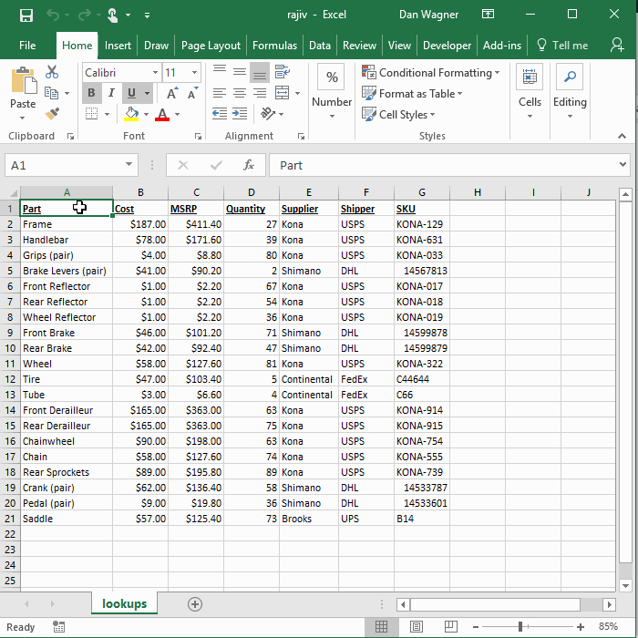
First, on line 9, we assign wksLookups to be the Worksheet everything is taking place on by taking advantage of the Range.Parent method.
Then, on line 12, we set the background color to ALL of column G to be the default “clear” (i.e. None). You might be asking yourself at this moment, “But why?”
Why are we doing this?
Another great question!
This line is a must to make sure we reset (or “initialize”) the highlight column, which is G in this case, back to a default state before applying the background change later on. If we did not initialize here, cells would remain highlighted even after the selection changed!
And with that, our Step 1 – Setup is complete. Let’s keep it moving y’all…
Step 2 – Exploration takes place on lines 17-22.
First, on line 17, we use an If statement to check two things:
Is Target in column A (i.e. column 1)?
Is the first row of Target 2 or greater?
This is because we are only interested in selections in column A, and because in this example row 1 is a header row.
(If you want row 1 to work like all the other rows, you can simply get rid of the And Target.Row > 1 portion of the If statement here.)
Next, we determine the first and last rows contained in Target on lines 21-22.
The first row is easy — we can simply call Target.Row to get the first row.
The last row, though, requires a bit more work. The built-in Range.Rows.Count method will give us the number of rows inside Target, but that number is relative and specific to wherever Target is. In this case, we need the absolute final row number.
To make sure we get the absolute final row number, we add the total number of rows in the Target Range to the first row number minus one like this:
Target.Rows.Count + (Target.Row – 1)
Nice!
That wraps up our Step 2 – Exploration, which means we’re ready to move on.
Step 3 – Execution is where the actual cell highlighting takes place, with lines 25-28 getting the job done.
First, on line 25, we use a context manager (With wksLookups) to make sure we don’t have to type the Worksheet variable a bunch of times.
Inside the With statement, on lines 26 and 27, we define the Range we want to highlight and set its background color to yellow.
This defines the Range that we will be highlighting.
Back on lines 21 and 22, we defined lngFirstRow and lngLastRow by taking advantage of some built-in methods on Target.
We know that column G (or column 7 if we’re talking numbers) is where we want to apply highlighting, so that is our column number in both of the .Cells(RowNumber, ColumnNumber) calls.
Next up, the actual background property:
.Interior.Color
When working with a Range variable, you can change the background color by using Range.Interior.Color = whatever.
And that whatever value here? Well, we are going to use the built-in RGB (Red Green Blue) function to make the color yellow with:
RGB(255, 255, 0)
And that’s it!
In this situation there is no Step 4 – Cleanup to be done, so we are finished!
Want to see this code in action? Here’s an 5-minute video guide:
Got your highlighting tool up-and-running like a boss? If not, let me know and I’ll help you get what you need! And if you’d like more step-by-step, no-bullshit VBA guides delivered direct to your inbox, join my email newsletter below.
There are many variations on the need here: maybe you need each new row in an output file to have a unique ID column, maybe you need to differentiate between orders from multiple tracking systems… the common thread here is needing something that is guaranteed* to be unique.
(*Note: yes, statistics zealots, I am aware that, assuming uniform distribution, there is a 50% chance that in a set of 4,200,000,000,000,000,000 GUIDs, there will be one duplicate… fuck off.)
Fortunately for us Excel and VBA users, generating a GUID with a function is a cinch:
Step 1 – Setup in this function is essentially just our variable declarations and assignments on lines 6-19. We create an Object variable, obj, which will be assigned to the built-in Scriptlet.TypeLib object, and a String, strGUID, which will contain the GUID.
Line 19 is where we assign obj to the Scriptlet.TypeLib object, but because this is a different notation than usual, let’s take a moment to talk about exactly what’s happening here.
Whenever you see:
in VBA, you are observing something called late-binding. Contrast this to early-binding, which looks like this:
If you have read some of my other tutorials, you will often see early-binding in use with the Scripting.Dictionary object:
There are many articles out there that contrast early-binding vs. late binding, and (surprise!) I have a strong opinion about it: use early-binding whenever you can. Period.
(You can write a check to the Dan Wagner Co. for saving you a half-day of reading :troll_smile:)
Unfortunately, in researching and testing the Scriptlet.TypeLib object, I could not figure out how to early-bind that sucker. It constantly throws “object or with block variable not set” errors, and does not even seem to be named the same thing!
Save yourself the struggle here and use late-binding, comfortable in the fact that this is literally the only time, in my years of VBA experience, I have found late-binding to be necessary.
Now that we have put Step 1 – Setup to bed, it’s time to move on.
Step 2 – Exploration is only line 22 here, where we assign strGUID to a manipulation of the .GUID method.
Interestingly, when calling obj.GUID, you wind up with a null-terminated string. This can be quite annoying depending on the application, so we use Left(obj.GUID, Len(objGUID) – 2) to get all characters EXCEPT the last two.
And with that, our Step 2 – Exploration is done!
The variable strGUID contains a full-fledged GUID, with hyphens and curly braces, that looks like this:
{88B6591C-053D-414E-8447-224704047786}
Wahoo! It’s time to move on to the next step.
Step 3 – Execution is where we (potentially) apply a few tweaks to strGUID, depending on how the function was called.
If you look at the function definition itself (which is on line 2), you’ll notice that there are two Optional Parameters:
IncludeHyphens, a Boolean variable, which is defaulted to True
IncludeBraces, a Boolean variable, which is defaulted to False
Optional Parameters are, exactly like the name implies, optional. They are not strictly necessary for the function to work!
There are two different ways to use Optional Parameters — one that sets them up as Variant-type and then tests for existence, and one that sets them up as specific-types and includes a default value.
The latter, where the Optional Parameters are configured as specific-types (Boolean in this case) with a default value, is what I recommend whenever possible. Testing for existence is a pain in the ass.
Let’s talk about how each one of these Optional Parameters works as part of our Step 3 – Execution.
The first is IncludeHyphens, which defaults to True. Hyphens are commonly included in GUIDs, but if you would like them removed, you can call this function with IncludeHyphens set to False instead.
On lines 26-28, we handle IncludeHyphens and the resulting strGUID change.
Remember, IncludeHyphens has a default value of True, so if you do not change that, Not True becomes False, skipping line 27.
If, however, IncludeHyphens was set to False, line 27 would be executed. If that is the case, then we replace all of the hyphen characters in strGUID with vbNullString, which is blank. Boom, hyphens removed.
The second Optional Parameter is IncludeBraces, which defaults to False.
A typical GUID does not include those opening and closing curly braces, so the function is set up to remove them by default (meaning that lines 33 and 34 are, by default, executed).
Much like line 27, we update strGUID with the Replace function, first replacing the open curly brace with vbNullString (blank), then replacing the close curly brace vbNullString (blank) as well.
Finally, on line 37, we set the function return to strGUID.
No clean up necessary, so we skip Step 4 – Cleanup — and with that, we’re done!
You can see how this function works inside the VBA editor by calling it a few times and writing the output to the immediate window like so:
Or, you can follow along with me in this 8-minute guide to the function, how to use it in the wild, and how adjusting the Optional Parameters can give you different results:
Are you creating GUIDs and writing them with ease? If not, let me know and I’ll help you get what you need! And if you’d like more step-by-step, no-bullshit VBA guides delivered direct to your inbox, join my email newsletter below.
But what about when you have different columns on each sheet? Or when the columns share similarities, but are in different order?
It’s a pain in the ass, but by using a Scripting.Dictionary to track column names (as Keys) and numbers (as Items) you can ensure that your data lines up appropriately for an easy pivot table.
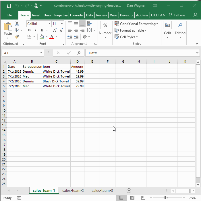
Let’s check out an example, featuring my favorite sales teams of all time: Dennis, Mac, Frank, Charlie, Sweet Dee, and Artemis from It’s Always Sunny in Philadelphia. You’ll notice that the sheets have some columns in order, some shared columns, and some NON-shared (i.e. totally different) columns:
Each sheet has similarities and differences in columns!
Cool!
Before we go any further, you will need to make sure you have the Microsoft Scripting Runtime added to this project (if you have not already).
This is how to add the Microsoft Scripting Runtime Reference
This 13-second gif walks you through the steps, but in case it is not working here is a quick step-by-step guide:
Open the VBA Editor window
Click “Tools” from the File menu
Select “References” from within the Tools menu
Scroll down until you find “Microsoft Scripting Runtime”
Check the box next to the “Microsoft Scripting Runtime”
Click OK
Phew! Now we can get back to the task at hand… combining data!
Here’s the scoop y’all — our It’s Always Sunny sales data can be combined with this macro:
Step 1 – Setup is a cinch, and we knock it all out on lines 14-18. We:
(line 15) Make sure the Scripting.Dictionary is set to vbTextCompare, which means the Keys will be case-INsensitive
(line 16) Assign lngFinalHeadersCounter to 1, since we do not have any column headers… yet
(line 17) Assign lngFinalHeadersSize to the .Count of dicFinalHeaders, because we will need to know when new columns are added (and will use this variable for comparisons)
(line 18) Create a new Worksheet and set it to wksDst — this will be our Destination Worksheet, where all of the data will be combined
Smooth! With our set up out of the way, we’ll accomplish Step 2 – Exploration and Step 3 – Execution in two phases:
Phase 1: assemble the final headers Scripting.Dictionary and prepare the Destination Worksheet
Phase 2: copy each column from each Worksheet to the appropriate place on our Destination Worksheet
Let’s dive into Phase 1!
The Step 2 – Exploration of Phase 1 takes place between lines 26-40.
First, we start looping through all of the Worksheets in ThisWorkbook on line 26, ignoring the Destination Worksheet (wksDst) on line 29.
Once we are sure we are NOT on the Destination Worksheet, we identify the last-occupied column on line 35 using LastOccupiedColNum from the VBA Toolbelt. You’re using the VBA Toolbelt, right? Please download it, use it as your new project template, and save yourself TONS of repetitive coding…
But let’s move on, as our Step 2 – Exploration for Phase 1 is done!
Line 36 kicks off a For…Next loop through this Worksheet’s occupied-columns, which is where our Step 3 – Execution takes place for Phase 1. Inside this loop, we will repeat the next 4 steps for each column header:
(line 40) Assign strColHeader to be the leading-and-trailing-spaces-removed column header name
(line 41) Check dicFinalHeaders to see if it already contains this column name (i.e. strColHeader)
(lines 42-43) If that column name is NOT in the Scripting.Dictionary from step #2 above, add it as the Key, with lngFinalHeadersCounter, representing the target column number, added as the Item
(line 44) Increment the lngFinalHeadersCounter variable so the next new column header name points to the next column number
Since we are inside the For Each wksSrc In ThisWorkbook.Worksheets loop, those steps are repeated for each Worksheet as well!
The last bit of Step 3 – Execution for Phase 1 happens on lines 58-60, which is where we set up the Destination Worksheet with the header column names we just collected.
Line 58 starts by kicking off a For Each loop to iterate through each Key in dicFinalHeaders.
Finally, on line 59, we write each header column name to its appropriate column number on wksDst, our Destination Worksheet — a cinch, since dicFinalheaders(varColHeader) gives us the column number.
Boom! That wraps up Phase 1 and sets us up for an easy Phase 2 — take a moment to celebrate and enjoy this gif of Charlie shooting a gun.
Get excited like Charlie y’all, we’re almost done!
The Step 2 – Exploration in Phase 2 takes place between lines 71-85.
Much like Phase 1, we use a For Each loop on line 71 to iterate through each Worksheet, and on line 74 we make sure that the final Destination Worksheet is skipped.
So far, so good!
On lines 80 through 85, we assign three variables to make our copy / paste (which is the next step in Phase 2, Execution) work smoothly:
(line 80) lngLastSrcRowNum is the last-occupied row on the Source Worksheet, which is where we will copy data FROM
(line 81) lngLastSrcColNum is the last-occupied column on the Source Worksheet, which determines the bounds of our (eventual) loop through all of the data columns
(line 85) lngLastDstRowNum is the last-occupied row on the Destination Worksheet, which is where we will paste data TO
That wraps Step 2 – Exploration for Phase 2, which means it’s time to jump into Step 3 – Execution!
Line 90 kicks off a For loop through each of the columns on our Source Worksheet. (Remember, we repeat this for each Worksheet that is not the final Destination Worksheet, just like in Phase 1.)
Line 91 assigns strColHeader, the name of this particular column header. (We will use this name in the next step, to get the right destination column number from dicFinalHeaders.)
Lines 95-96 set rngDst, the cell target on our final Destination Worksheet, using two things:
lngLastDstRowNum + 1, since we want to send our data one row below the last-occupied row on the Destination Worksheet
**dicFinalHeaders(strColHeader), which as you know will return the appropriate column number
Easy peasy!
Lines 97-98 set rngSrc, the column of data from our Source Worksheet. Since we know the column number (lngIdx, as we’re looping through the columns) as well as the last-occupied row on the Source Worksheet (lngLastSrcRowNum), we can create this Range using these cells.
And finally, the copy / paste happens on line 104, where we call the Copy method on rngSrc with a Destination parameter of rngDst.
And with that, you’re done! Time to celebrate y’all, as you have solved a seriously challenging problem in a VERY flexible way.
We did it you guys, we did it!
The last little bit of this script is our Step 4 – Cleanup, which takes place on line 115. All we’re doing here is throwing a MsgBox to the user, letting him or her know that the data has been combined. Wahoo!
Want to see this code in action? Here’s a 12-minute guide to the script, most of which is spent illustrating exactly how each column of data gets lined up appropriately on the Destination Worksheet:
Are you combining multiple Sheets with out-of-order (or completely different) columns into a single Sheet like a pro? If not, let me know and I’ll help you get what you need! And if you’d like more step-by-step, no-bullshit VBA guides delivered direct to your inbox, join my email newsletter below.
Anyone who tells you they didn’t love this song is lying
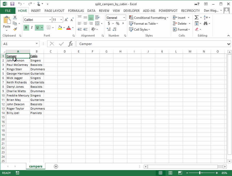
How do you determine whether an object is a member of a Collection?
Folks with experience in other programming languages would probably assume that this functionality is built into VBA… And unfortunately, those folks would be wrong.
If you need a BULLETPROOF way to see if your Collection contains something (like a String, a Range, a Worksheet, etc.) look no further! The following Contains function:
Attempts to find the object using a Key
If no Key is provided, it loops through the Collection, checking each Item
If no Key or Item is provided, it defaults to False
The Step 1 – Setup in this function is minimal, and takes place entirely on lines 9 and 10 with the declaration of our variables: strKey and var. More on them later!
Step 2 – Exploration comes up in a hurry. Much like the set up, our Exploration phase is really short — in fact, it is essentially a single If / ElseIf / Else statement!
This statement starts on line 13, where we check to see if a Key was passed-in to the function. The ElseIf statement starts on line 39, where we check to see if an Item was passed-in to the function. Finally, on line 50, we default the Contains function to False if no Key or Item was passed-in. Easy cheesy!
So far so good!
Step 3 – Execution is where things start to get interesting. As we said earlier, there are three branches our code can take:
If the user passed-in a Key, we’ll use that to check the Collection
If the user passed-in an Item, we’ll loop through the Collection, checking each contained item to see if it matches the passed-in Item
If neither a Key or an Item is passed in, we return False by default
Let’s start with the easiest one first and work our way up!
3. If neither a Key or an Item is passed-in
This one’s a cinch. If the user calls Contains without passing in a Key or Item, we return False — lines 52 and 53 take care of that. Done!
2. If the user passed-in an Item
If the Collection in question does not make use of the (admittedly optional) Key parameter, then we will need to loop through the Collection and check each of its items against the passed in Item.
We tackle this on lines 41-49.
We start on line 41 by assuming that the passed-in Item will not be found, meaning Contains will return False. Don’t worry — we’ll set Contains to True if we do find the passed-in Item!
Collections support the For Each…Next loop construct with a Variant-type iterator, which we kick off on line 44. (That’s the var variable in this case.)
On line 45, we are checking each item (var) in the Collection to see if it matches the passed-in Item. As soon as a match is found, we set the Contains function to return True (on line 46) and exit (on line 47)!
1. If the user passed-in a Key
Jackpot — this one is absolutely the most fun of all, and it executes between lines 15 and 36.
The first thing we do is convert Key, which is technically a Variant, into a String on line 15. (Collections only allow for String-type keys, but we declare the optional input Key as Variant to allow the user to skip it if need be.)
Take a deep breath y’all — we’re about to enter Error Handling country…
On line 18, we use On Error Resume Next to ensure that VBA does not stop executing the code if an Error occurs. Why though?
Why are we using On Error Resume Next?
Fortunately for us, the assignment on line 20 will (potentially) generate very predictable errors.
We start off this section by assuming the Key will be found, which is why we set Contains to True on line 19.
On line 20, as mentioned a moment ago, we attempt an assignment that might generate error.
On line 21, we check to see if Err.Number is 91 (which means an error occurred and the error number is 91). If so, the assignment itself failed! VBA throws this error when you attempt to assign an object without using the Set keyword — for example, if you wrote wks = ThisWorkbook.Sheets(1) instead of Set wks = ThisWorkbook.Sheets(1).
If the assignment failed, we jump to line 26 (CheckForObject), where we use the IsObject function on line 27 to properly check if an object (like a Worksheet or Workbook, for example) is stored in the Collection. If so, we can set Contains to True and exit!
What if we did not get error 91 though, and instead got error 5? (The error 5 case is what we are checking on line 22.)
VBA will throw a 5 error when the specified Key is not found in the Collection. In that case, we jump to line 33, where we set Contains to False and exit. Nice!
What if neither error 5 nor error 91 occurred? Well, in that case, we reset the error handling with On Error GoTo 0 on line 23 and exit the function with Contains still set to True, the way it was on line 19.
Phew! For such a small task, there were many edge cases to consider — fortunately, covered them all here and can use this function with confidence!
If you’d like to do some of your own checking on the Contains function, you can use my comprehensive test file to be 100% sure about how Contains works:
In the 9-minute video below, I do exactly that — walk through each test case!
Checking collections with confidence? If not, let me know and I’ll help you get what you need! And if you’d like more step-by-step, no-bullshit VBA guides delivered direct to your inbox, join my email newsletter below.