
How to Combine Data from Multiple Sheets into a Single Sheet
How do I fill-in sheet 1 with data from sheets 2, 3, 4 … ?

It’s time to combine data y’all
Like Samuel L. Jackson in Jurassic Park, this one’s a classic. You and your team are sharing a single Workbook, with each of you operating on your own Sheet. Once everybody is done, you need to combine the data from each Sheet into a single, continuous Sheet for import into a different program. (Or a final pivot table. Or a report to your manager. Or a what-the-flip-ever …)
Let’s dissect a real example. Suppose you have a Workbook like this, with data Sheets that have the same headers (but different info on each). You want to combine this data onto the “Import” sheet, which has the exact same headers too.
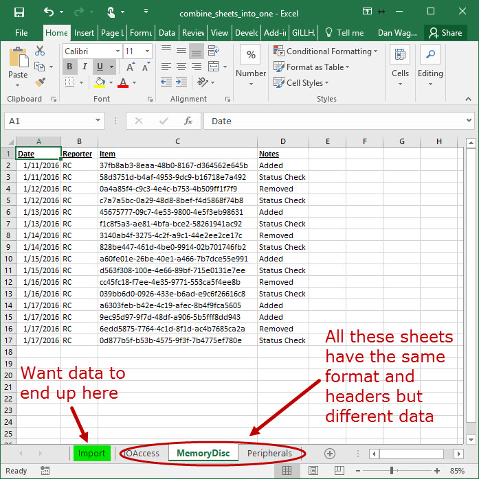
All Sheets have the same headers but varying rows
Cool. Here’s the code that gets the job done:
Let’s review the code using our 4-step VBA process as a guide:
Step 1 – Setup
Step 2 – Exploration
Step 3 – Execution
Step 4 – Cleanup
Step 1 – Setup takes place from lines 11-13, where we make three assignments:
- wksDst, the “Import” Worksheet
- lngDstLastRow, the last-occupied row on the “Import” Worksheet
- lngLastCol, the last-occupied column on the “Import” Worksheet
We know that all the data Worksheets have the same shape, so lngLastCol is going to be the same value for the duration of the script.
(Wondering about the functions LastOccupiedRowNum and LastOccupiedColNum? They’re in the VBA Toolbelt and are also defined on lines 45-87… You will use these functions constantly in Excel, so get used to defining them in your macros!)
The final setup step occurs on line 16, where we assign the initial Destination — this is where our first paste will start.
Next up is Step 2 – Exploration, which occurs inside the loop from lines 19-25. The For Each wksSrc in ThisWorkbook.Worksheets loop iterates through all Worksheets in this Workbook. (LOVE this syntax… so easy to read and understand!)
Line 22 ensures that the “Import” Worksheet is skipped (since that Worksheet is the destination, NOT a source). This phase ends on line 25, where the last occupied row on the source Worksheet is identified — again, leveraging LastOccupiedRowNum from the VBA Toolbelt.
We’re onto Step 3 – Execution! Short and sweet here, from line 28 to 31.
The source Range is assigned on line 29, taking advantage of the last row, lngSrcLastRow, which we figured out on line 25 above, and lngLastCol, which we identified wayyy back up on line 13. Finally, we use the Range.Copy method on line 30 to move the data to the destination Range — smooth!
Lines 34-35 are a quick switch back to Step 2 – Exploration, this time taking place on the destination (“Import”) Worksheet. Since new data has been added (in the Execution step above), we recalculate the last-occupied row, reset the destination range and continue the loop on to the next Worksheet.
That’s it, no Step 4 – Cleanup necessary!
Here’s a 4-minute guide to the code above, with an emphasis on the Exploration and Execution steps:
Combining multiple Sheets into one Sheet with VBA like a boss? If not, let me know and I’ll help you get what you need! And if you’d like more step-by-step, no-bullshit VBA guides delivered direct to your inbox, join my email newsletter below.