How can I use VBA to calculate and label all the duplicates in a given range in a way that’s faster than using COUNTIF or Range.Find?
Sometimes it’s all about speed you guys
When you’re dealing with large data sets (say +250K rows), speed matters.
Let’s say you have 322K rows with IDs. There are about 2000 IDs that show up only ONCE in the data, and the rest come up more than once — we want to find and label all of the IDs that only occur once.
The high-level strategy for this uses two Scripting.Dictionary objects, which I’m going to shorten to just “Dictionary” for the rest of this tutorial:
Create a Dictionary of distinct IDs (dicDistincts)
Create a Dictionary of IDs that occur more than once by using the Dictionary from step #1 — these are our duplicates! (dicDuplicates)
Loop through all the IDs, marking IDs that are found in the duplicates Dictionary (dicDuplicates) as “Duplicate” and all others as “Unique”
Before we dive in, though, you need to make sure you have the Microsoft Scripting Runtime added to this project!
This is how to add the Microsoft Scripting Runtime Reference
This 13-second gif walks through the steps, but in case it stops working:
Open the VBA Editor window
Click “Tools” from the File menu
Select “References” from within the Tools menu
Scroll down until you find “Microsoft Scripting Runtime”
Check the box next to the “Microsoft Scripting Runtime”
Click OK
Jackpot — you now have access to the Dictionary object! Let’s return to our regularly-scheduled programming…
We’re labeling uniques and duplicates here, and the super-commented code below does exactly that:
All of the Step 1 – Setup takes place on lines 21 through 29.
First, we assign wksIDs on line 20 to make it easy to reference this Worksheet. On line 21, we quickly find the last-occupied row and store it in lngLastRow using LastOccupiedRowNum — one of the staples of the VBA Toolbelt. (You’re using the VBA Toolbelt, right? If not, get it here.)
Let’s take a minute to closely review lines 22 and 23, where the CompareMode property of each Dictionary is set to vbTextCompare.
Why mess around with the CompareMode property?
Dictionary keys in VBA default to CASE-SENSITIVE, which is something we would like to avoid here. In order to ensure a Dictionary ignores the difference between upper and lower case letters, you must set the CompareMode property to vbTextCompare like we do on line 22 and 23.
Finally, on lines 26 and 30, we create Variant Arrays representing the IDs themselves (varIDs) as well as the status of the IDs (varStatus), which will be “Unique” or “Duplicate”.
Since we know varStatus will be exactly as long as varID (each row needs to be labeled “Unique” or “Duplicate”), we initialize it to simply match varIDs to start.
Phew! We’re done with our Step 1 – Setup, and that means it’s time to start exploring this bitch.
Step 2 – Exploration takes place between lines 34 to 58, which is a single For Each loop through the Variant Array containing the IDs (varIDs).
First, on line 37, we assign the ID to a handy short variable, strID, using CStr to convert it to a String then leveraging Trim to remove any leading or trailing spaces.
Line 40 is essentially a guard clause. We don’t care about blank IDs, so we skip them.
The magic really starts between lines 44-54!
We initially check the distinct Dictionary (dicDistincts) to see if the ID has already been observed by using the Dictionary.Exists(Key) method, which returns a handy True or False.
If this particular ID is NOT already in the dicDistincts Dictionary, we add it.
If this particular ID is already in the dicDistincts Dictionary, we know we have a duplicate! In that case, we attempt to assign it to the duplicate-containing Dictionary, dicDuplicates.
Once again, on line 52, we check to see if this value already exists in the Dictionary. If so, we do nothing except move on to the next loop.
Wahoo! We’re done with the Step 2 – Exploration and will be diving into our deceptively simple Execution step.
Step 3 – Execution takes advantage of the dicDuplicates, the Dictionary we assembled on line 53, that contains every ID that is repeated. By working through the full column of IDs and checking to see if that ID exists in dicDuplicates, we can easily label the “Duplicate” and “Unique” IDs!
Step 3 – Execution kicks off on line 69, where we start by setting the lngIdx variable to 1. (We’ll be using this variable as a counter as we walk down the Variant Array containing all IDs.)
Line 70 is where we start looping through all of the IDs contained in the Variant Array containing them, varIDs. At each step, we check to see if this ID exists in the duplicates Dictionary, dicDuplicates, by using the Dictionary.Exists method, which returns True or False depending on (you guessed it) whether or not the ID is there.
If the ID exists in dicDuplicates, we know we’re dealing with a dupe — and that means setting the value in varStatus, the Variant Array we created to label each ID, to “Duplicate (on line 72). If dicDuplicates does NOT contain the ID, then we know it’s unique and label it as such!
Now that varStatus has “Unique” or “Duplicate” for every ID, all that’s left to do is write those contents out to the Worksheet, which we handle on line 80. Jackpot — our Execution step is done!
Not much to mop up here, so Step 4 – Cleanup is simply a message box letting the end user know that the macro is finished.
(In this particular case, I included a little timer to make sure the performance was good — that’s why you see dblStart and Timer in the mix.)
Daaaamn that was fast!
Here’s an 8 minute YouTube video demo and walkthrough that compares the performance of this method as well as an alternative, then covers the finer points from above:
Identifying and labeling uniques and duplicates with ease? If not, let me know and I’ll help you get what you need! And if you’d like more step-by-step, no-bullshit VBA guides delivered direct to your inbox, join my email newsletter below.
Insert rows without ball-ache by following the steps below
Actually inserting rows with VBA is easy enough, but getting the logic right, ESPECIALLY inside a loop, can be a pain in the dick!
This is because the default loop behavior is to start at the top (small row numbers) and end at the bottom (big row numbers). When adding rows, however, each addition changes the underlying row indices on the Worksheet!
Unless you have accounted for that change (you haven’t, by the way), the logic inside your loop is going to act on the wrong rows after the first new row is inserted… and that’s a recipe for disaster.
The solution? Work “backwards”, from the bottom to the top.
Let’s check out an example.
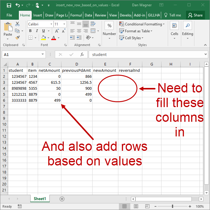
This is the sheet we start with
Suppose that we need to fill-in the newAmount and reveralInd columns, and we also need to add rows based on the value of netAmount.
Here are our rules:
newAmount should always be set to the same value as previousPdAmt
reversalInd should always be set to “Y” with one exception (#7 below)
If netAmount is greater than zero, we need to add a row immediately below the greater than zero occurrence
In the newly-added row, the student should be the same as the above
In the newly-added row, the item should be the same as the row above
In the newly-added row, the newAmount should be set to the netAmount from the row above
In the newly-added row, the reversalInd should be set to “N” (this is the one exception we mentioned in item #2)
Sounds like a lot, but by following the “go backwards, from bottom to top” strategy we’ll make short work of this job.
In this case, Step 1 – Setup and Step 2 – Exploration are essentially the same thing (since we already know the column numbers). These steps take place on lines 13 to 21.
Lines 14-19 handle the column numbers for each field, from student all the way to reversalInd.
Line 20 is where we assign the Worksheet containing all our data. And finally, line 21 is where we identify the last-occupied row on the data Worksheet using the super-handy LastOccupiedRowNum from the VBA Toolbelt. You ARE using the VBA Toolbelt, right? If not, take 7 seconds and get it here.
That’s it! With Step 1 – Setup and Step 2 – Exploration out of the way, we jump into Step 3 – Execution.
This takes place between lines 23-69, which we’ll split into two phases:
(Phase 1) apply logic from above AND identify rows where we’ll need to insert a new row
(Phase 2) insert new rows per Phase 1 and apply the rest of the logic from above
Sound like a plan? Cool — let’s get after it then.
Phase 1 of Step 3 – Execution is the For loop that takes place on lines 26-41. Note the structure of this For loop — we start at the last row (lngLastRow) and work BACKWARDS to 2, decreasing the counter (lngIdx) by 1 each time!
Based on the logic from above, lines 31-32 handle the first two rules:
(line 31) newAmount should always be set to the same value as previousPdAmt
(line 32) reversalInd should always be set to “Y” with one exception
Lines 37-39 use a Collection to identify any row where the netAmount is greater than zero. We do this to accomplish the goal set out in rule #3:
If netAmount is greater than zero, we need to add a row immediately below the greater than zero occurrence
Again, since we are working backwards (from the bottom to the top), it’s important to know the row numbers will be stored in this Collection from largest to smallest! This strategy will come in handy in Phase 2, which occurs below.
Phase 2 of Step 3 – Execution is the For Each loop on lines 51-67.
First, though, a short note on the actual structure of this loop. In general, I prefer “For Each” loops over “For” loops — by picking a good iterator variable name, “For Each” loops practically read like perfect English! Code that reads like English is easy for your coworkers to understand, which means the code will also be easy to maintain.
Since collections in VBA can be iterated through using For Each (with a Variant-type iterator), that is the strategy we’ll be using here.
Since each item in the Collection is a row number where a new row must be inserted (sorted from largest to smallest), our first task is to insert those new rows! This occurs on line 54.
Lines 57-58 accomplish rules #4 and #5:
In the newly-added row, the student should be the same as the above
In the newly-added row, the item should be the same as the row above
Since we know varRowNum is the row immediately preceding the just-inserted row, we can access the just-accessed row number with varRowNum + 1. This is exactly how we’ll work on this new row for every applicable rule!
Speaking of rules, we accomplish rule #6 with line 62:
In the newly-added row, the newAmount should be set to the netAmount from the row above
And finally, we follow rule #7 on line 65:
In the newly-added row, the reversalInd should be set to “N” (this is the one exception we mentioned in item #2)
That’s it for Step 3 – Execution!
There is not much to clean up here, so Step 4 – Clean Up is simply an alert to the user (on line 72) letting him or her know that we’re done. Sweet!
By working backwards, from bottom to top, we can insert rows without any complicated row-number-shifting techniques… and when it comes to VBA code, simple is good.
More of a visual learner? No worries! Here’s a quick 7 minute run-through of this technique on the code on YouTube:
Inserting rows based on values with the precision of a Jean-Claude Van Damme Bloodsport kick? If not, let me know and I’ll help you get what you need! And if you’d like more step-by-step, no-bullshit VBA guides delivered direct to your inbox, join my email newsletter below.
Then, from line 16 to line 21, we initialize “ALPHA”, the destination sheet. If the last-occupied row on the destination sheet is greater than 1 (i.e. the header row), then we know some data already exists. In that case, we use the Range.ClearContents method to get rid of that data in preparation for adding the individual days’ data.
Finally, on line 25, we assign the initial destination range (rngDst) — and with that, our setup is complete!
Next up is Step 2 – Exploration, which runs from lines 29 to 46.
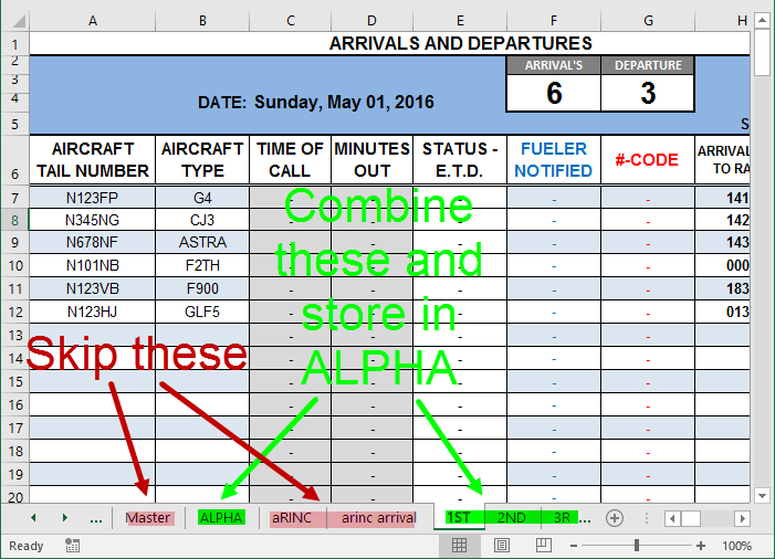
The For Each…Next loop that begins on line 29 allows us to iterate through each Worksheet, which is stored in wks. This means that on each cycle of the loop, wks will be set to a different Worksheet in the file.
First, we use the Worksheet.Name method to store the upper case name of wks in strName, which makes for a very easy-to-read next step.
We know that we need to skip any Worksheet that is not “1ST”, “2ND”, “3RD”, etc., so we check each name using a multi-line If statement in lines 34-39.
Assuming that wks is NOT one of the Worksheets to be ignored, Step 2 – Exploration wraps up on line 46. Here, the last-occupied row on the Worksheet is identified and stored as lngSrcLastRow.
Wahoo — exploration complete!
We then move into Step 3 – Execution, which runs from lines 50-59.
Using lngSrcLastRow, the last variable we assigned in the exploration step, we assign the data range to rngSrc on line 51.
In this particular example, we only want the values and formulas from each data Worksheet. With that as our guiding princple, lines 52-54 take care of the job.
Line 52: Copy the source data using the Range.Copy method
Line 53: Paste to the destination using the Range.PasteSpecial method, first sending over the values and number formats ONLY
Line 54: Paste to the destination using the same method of #2 above, this time sending over the formulas ONLY
Nice!
Now that this particular Worksheet’s data has been copied to the destination, we need to update the destination range to match the new bottom of the data block.
This occurs on lines 58-59, where we use LastOccupiedRowNumInCol again (seriously, get the VBA Toolbelt), then set rngDst to reflect this new last occupied row.
Jackpot — that’s it for execution!
There isn’t much Step 4 – Cleanup to do in this case, so we simply let the user know all the data has been combined with a MsgBox on line 66.
And with that, we have successfully combined certain Worksheets while skipping others! In case you prefer video, here’s a 7-minute screencast walking through these steps:
Are you combining some and skipping other Worksheets with the best of them? If not, let me know and I’ll help you get what you need! And if you’d like more step-by-step, no-bullshit VBA guides delivered direct to your inbox, join my email newsletter below.
Evan and I taking notes from the original Regulators
Did you know that Excel does not have a built-in MEDIANIFS function? You know, like AVERAGEIFS or SUMIFS, just with a median calculation instead of an average or a sum? Your boy didn’t, that’s for sure.
Which is why I’d like to give a HUGE shout to Evan at Mosaic Ventures. Like a gangster, Evan:
Identified the missing MEDIANIFS function in the first place
Commissioned a VBA-based implementation
Gave me the OK to release the code to everyone + dog
Fuck yeah Evan. You’re a renaissance man.
Full disclosure you guys — the ~200 lines below are advanced, but heavily commented. Read through the comments and the process will crystallize in your mind grapes — scout’s honor.
More importantly, the logic for identifying which cells to consider and which to throw away is universal. What does that mean for you?
If you want to, say, build a MODEIFS instead of a MEDIANIFS, you simply have to change ONE LINE. That’s it. One.
So with that in mind, let’s flex those code muscles a little bit:
To start, Step 1 – Setup is actually minimal. The only real “setup” that we do before getting into step 2 takes place on line 7, where we re-dimension varAccumulator, which will store the values we want to take the median of, to be a single element in size.
Step 2 – Exploration starts with three guard clauses, occupying lines 10 through 36. Let’s cover each of them:
If the user mistakenly passes in an empty Range, we want the function to return 0
If the user mistakenly passes in a mismatched number of Range / Criteria pairs, we want the function to return 0
If the user mistakenly passes in Ranges that have different numbers of rows or columns, we want the function to return 0
Check #1 takes place from line 15 to line 18. If the median_range, which is passed-in by the user, is Nothing, we assign the output to be 0 and exit the function. Boom.
Check #2 takes place on lines 22 through 25. Every Range the user passes in (like A2:A30) needs to have a Criteria (like “<250”) — this means that there should be an even number of elements in range_and_criteria_pairs. (The name is a giveaway, after all.) We validate that this is true by subtracting the lower bound of the passed-in ParamArray variable range_and_criteria_pairs from the upper bound and making sure the result is an ODD number.
Tricky, right!? Let’s do a quick thought experiment to see why this is correct.
Suppose the user passed in C2:C30 as the Range and “>=5000” as the Criteria. In that case, ParamArray(0) is the C2:C30 Range and ParamArray(1) is “>=5000”. The upper bound is 1 and the lower bound is 0. 1 minus 0 equals 1, which IS evenly divisible by 2 — meaning that our check passes!
On the other hand, suppose the user passed in C2:C30 as the first Range, “>=5000” as the first Criteria, and D2:D30 as the second Range, but forgot to enter a second Criteria. In that case, the upper bound is 2 and the lower bound is 0. 2 minus 0 equals 2, which IS evenly divisble by 2 — meaning our check fails! Phew!
Check #3, the final guard clause, is on lines 30 through 36. For the MEDIANIFS function to work correctly, all of the passed-in Ranges need to be the same size and shape. (This is the case for SUMIFS and AVERAGEIFS too.) Verifying that, fortunately, is a snap — on line 31 we simply validate that the number of rows and columns in the passed-in Ranges match the number of rows and columns in the median_range, which was passed-in by the user and holds the column he or she would like to see the median of.
Wahoo! You’ve already come a long way, so take a second to celebrate. Seriously — that was some heavy data validation! Hats off to ya 🙂
Our Step 2 – Exploration begins in a new direction on line 43, where we start looping through all of the rows that are potentially going to be added to our median calculation.
Upon entering this loop, we immediately initialize blnAllMatched to False. We will use blnAllMatched to quickly identify situations where the Criteria is not met — but before then, we need to figure out what kind of operation (like less than or equal to) we’ll be conducting, as well as the threshold (like 200 or “Apples”) for that operation, for each Range / Criteria pair! On line 49, we start looping through the range_and_criteria_pairs, since the user can pass in as many as he or she would like.
For each Range / Criteria pair, we run through the beast mode Select Case statement from line 52 to line 96 to identify the operation (like less than or equal to) and the threshold (like 200 or “Apples”).
This Monster Case Statement…
Lines 53 to 58 are very straightforward — if the first two characters of the Criteria string are less than or equal to, greater than or equal to, the operator (stored in strOperator) is assigned and the threshold (stored in varThreshold) is extracted.
Lines 62 through 69 handle the not equal to sign. As indicated by the comments, this is a little tricky — the user could be trying to match a number (like “<>200”) or a string (like “<>Apples”)! To handle both cases, we use the handy IsNumeric built-in function (as well as the equally-handy IsEmpty function, since IsNumeric evaluates to true on empty cells) on lines 64 and 65.
Lines 74 through 79 function the same way as the first two clauses of the our original Select Case statement — if the first character of the criteria string is less than or greater than, we again assign the strOperator variable and extract the varThreshold.
Lines 83 through 89 handle the equal sign, which is tricky — just like the not equal to sign. We use the same IsNumeric / Not IsEmpty strategy here on lines 85 and 86 to tell the difference between numbers and strings.
Finally, lines 95 to 102 handle everything else. Just like the comments say, we’re going to bucket everything else as an equality check — fortunately, this means that we can use the exact same logic from the equal sign check! (The only difference is that in this case we do not need to chop off the equal sign character.) Nice!
Hell yeah! At this point, you have an operator (stored as strOperator) and a threshold (stored as varThreshold) — all that’s left to do is check the cell value against the operator and threshold! This is where the blnAllMatched variable comes in handy too.
At last y’all, it’s time for Step 3 – Execution, which occurs between lines 108 and 189. Let’s get it…
Once again, we’re going to use a Select Case statement from lines 111 to 160 — this time, though, we’re checking the strOperator variable, applying logic as needed.
On line 112, for example, we handle “<>” (does not equal) by checking the cell value to see if it is not equal to varThreshold — if so, blnMatched is set to True because that Range / Criteria pair was successful!
Line 118 handles “>=” (greater than or equal to) the exact same way — same for line 124 (“>”, greater than), line 130 (“<=”, less than or equal to), all the way through the end of the Select Case statement on line 161. In fact, you might even be thinking that this section is very similar to the last section of Step 2 – Exploration — and you’d be right!
Line 168 is critical here you guys, so listen up. If blnAllMatched is False at the end of a check for ANY Range / Criteria pair, we know that this cell will NEVER be added to median calculation! If that’s the case, we can break the Range / Criteria loop (which is using lngCriteriaIdx) and move on to the next row.
Almost there you guys! Lines 174 through 181 handle value accumulation — let’s break that down.
On line 174, we check to see that blnAllMatched is True. If so, we know that every Range / Criteria check was successful, so we’re PROBABLY going to add the median_range value to our accumulator array, varAccumulator.
On line 176, we make sure that the value from median_range is numeric (since you can only calculate a median on numbers) and not empty (again, since you can only calculate a median on numbers). If the value passes those checks, we add it to the end of varAccumulator, then increase the size of varAccumulator by one on lines 177-178.
Once we get to line 186, our code has worked its way through every row! Since the last time a value was added to varAccumulator we increased its size by one, we know that the last element is empty — which is why we chop it off.
Finally, we take advantage of WorksheetFunction.Median, which calculates the median of varAccumulator like a champ. This is where you can substitute any statistic you’d like — for example, if you want to get the mode instead of the median, simply call WorksheetFunction.Mode instead! So right, so tight…
(The last few lines, from 193 to 201, are “nice to haves” — they add a description to the MEDIANIFS function and drop it into the “Statistics” group.)
PHEW! That was a lot. In case you’d like a visual review, here’s a 12-minute video of me walking through the same steps and demo-ing the new functionality:
Is your MEDIANIFS function humming along? Are you remixing it to build a different IFS function? If not, let me know and I’ll help you get what you need! And if you’d like more step-by-step, no-bullshit VBA guides delivered direct to your inbox, join my email newsletter below.
I recently saw an EXCELLENTLY-described question about converting semicolon-delimited TXT files to XLS (i.e. Excel 2003 and previous) format files that was unfortunately posted to StackOverflow. (I have a love / hate relationship with StackOverflow.) The reaction was your typical passive aggressive down-voting and eventually the question was closed. Sigh.
Converting delimited text files into Excel files is something you’ll probably do 50 times this year alone — which means it’s ABSOLUTELY worth solving in a smooth, repeatable way.
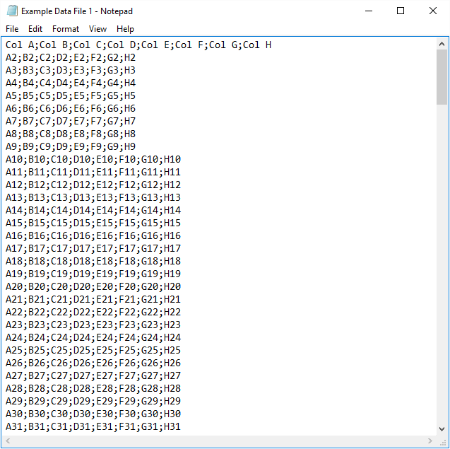
Suppose you need to convert many semicolon-delimited text files into XLS files, just like my bruised and beaten friend over at StackOverflow. The files look like this:
Before you get TOO lathered up about the length, know that lines 43 to 140 are already written for you in the Toolbelt, so we’re only going to focus on lines 1-41 (the ConvertSemicolonTextToXLS subroutine):
The Step 1 – Setup phase is handled entirely by lines 13 through 17 — the awesome PromptUserToSelectFiles function from the VBA Toolbelt mentioned earlier in this tutorial. Essentially, you only need to pass it 3 things:
AllowMultiples (Boolean): if you’d like the user to be able to select more than one file, set this to True — otherwise set it to False
DisplayText (String): this is the message you’ll see on the Windows Explorer prompt — here we set it to strMessage, which was assigned to “Please select the target semicolon-delimited TXT files” on line 13 above
TargetFileType (String): this allows you to limit the select-able file type to, say, just text — this function supports “XLSX”, “XLSB”, “XLSM”, “XLS”, “CSV”, “TXT”, and “ALL”
The PromptUserToSelectFiles function returns a FileDialog object, which we assign to variable fdoUserPicks on line 14. So much work accomplished in this little one-liner!
Finally, we’ll check fdoUserPicks to see if it is Nothing on line 17 — this is to catch a user clicking “Cancel” on the Windows Explorer window that was prompted on line 14… and with that, the Setup phase is done. Whaddupppppp!
Next up is Step 2 – Exploration, which is just line 20 in this case! Since there are (potentially) many filepaths in the fdoUserPicks object, we use a For…Next loop to cycle through them.
Step 3 – Execution takes place from lines 25 to 35. We start with the incredibly handy Workbooks.OpenText method, which handles parsing delimited files almost exactly like Range.TextToColumns. The Workbooks.OpenText method has lots of optional parameters, but in this case we really only need two things:
The filepath: since fdoUserPicks.SelectedItems holds the filepaths as strings, we get at each individual filepath by writing fdoUserPicks.SelectedItems(lngIdx)
Semicolon: just like Text to Columns inside Excel, semicolon is one of the named delimiters, so we simply need to set this parameter to True
If you’re dealing with a less common delimiter, like pipe “|” characters, fear not: you just need to set Other to True (Other:=True) and OtherChar to the character you need (OtherChar:=”|”).** I go more into detail on this in the video walkthrough below.
The Workbooks.OpenText method leaves the just-opened file as ActiveWorkbook, so on line 27 we set wbkData as such. Usually ActiveWhatever should be avoided, but because we KNOW Workbooks.OpenText works this way we’re in the clear.
Next up, a little file name prep on line 30. Whenver you need to remove X characters from the end of a string, this is the way:
Left(TheString, Len(TheString) – X)
Boom! We want to remove “.txt”, 4 characters, so our assignment looks like this:
Finally, on lines 34 and 35, we save the file in XLS format and close it. That wraps up the execution phase!
Our Step 4 – Cleanup is a breeze on line 39 — we simply let the user know that everything has been converted! And with that, the conversion is done.
More of a visual learner? Here’s an 8-minute rundown of the code, how it works, and how you can tweak it to handle less common delimiters (like the pipe “|” character):
Are you making short work of file conversion jobs? If not, let me know and I’ll help you get what you need! And if you’d like more step-by-step, no-bullshit VBA guides delivered direct to your inbox, join my email newsletter below.
P.S. the OP at StackOverflow figured out how to solve his problem and updated the question with “NEVER MIND – I FIGURED IT OUT” and a working solution! Maybe there is hope after all…