When you’re using Excel to track activities on a calendar, it can be incredibly helpful to highlight sections of the grid based on the cell you selected. If you need Excel to do something based on a selection, you should reach for the Worksheet_SelectionChange event.
Suppose your calendar looks like this, and you know that you can only go biking on Mondays, swimming on Tuesdays, and rowing on Wednesdays. Scheduling those activities would be easy cheesy with a visual aid in the form of changed background colors:
Using Worksheet_SelectionChange makes this a snap
So how does it all work? This short script is all you need:
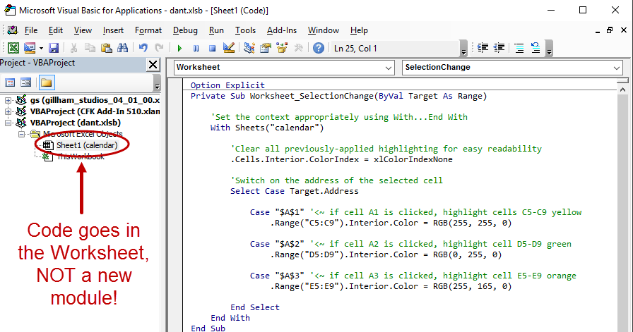
One CRITICAL note before we get into the details. In contrast to your typical VBA subroutine, we’re using an Event that’s tied to a Worksheet. (In this case, the Worksheet is “calendar”, but it could be any Worksheet.)
When you are taking advantage of Events, your code will go into the appropriate Worksheet (or Workbook) rather than a regular module!
This Event is tied to calendar, so the code belongs in the calendar Worksheet module
Step 1 – Setup takes place on lines 5 through 8. First, on line 5, we set up a context manager using With…End With, since we want to operate on the calendar Worksheet. Then, on line 8, we remove all cell highlighting from the calendar Worksheet to ensure a clean slate before moving on to the next steps.
Step 2 – Exploration is contained entirely within the Select Case statement that starts on line 11. Target is the Range passed in to Worksheet_SelectionChange and represents the cell our user clicked on, so we do our Select Case checking on Target.Address.
Line 13 checks to see if cell A1 was selected, line 16 checks to see if cell A2 was selected, and line 19 checks to see if cell A3 was selected. The Select Case statement is perfect for this situation since we need to check lots of potential cases and do not want to constantly be writing “If Then ElseIf Then ElseIf Then ElseIf Then …”
Step 3 – Execution happens inside each of the case options within the Select Case statement. Line 14 highlights cells C5:C9 yellow if cell A1 was selected, line 17 highlights cells D5:D9 green if cell A2 was selected, and line 20 highlights cells E5:E9 if cell A3 was selected.
Phew — with that, you’re done!
Here’s a 6 minute overview of the code including a demo of each activity for all the visual learners out there:
Are you highlighting destination columns in a way that will delight your users? If not, let me know and I’ll help you get what you need! And if you’d like more step-by-step, no-bullshit VBA guides delivered direct to your inbox, join my email newsletter below.
It condenses many lines of code and logic into a convenient single line
It has a name that describes exactly what it does
It lets you make a code change in a single place instead of multiple places, a concept commonly referred to as D.R.Y. (Don’t Repeat Yourself) in the development world
Heaven help you if the code is scattered in many workbooks
But there is a bulletproof strategy for writing Functions in VBA. Even if you use this technique to create just a few re-usable Functions (or Subroutines), the nature of the method guarantees that you will get a lot of mileage out of the results.
But that’s enough hype — let’s get to it.
Every time you copy / paste code in the VBA editor, ask yourself:
Am I doing the same thing here (paste) that I was doing there (copy)?
If the answer is “yes”, it’s time to write a Function or Subroutine!
Beautiful. Now that you know you’re doing the same thing in at least two places, these two questions will send you down the right path:
Does the copied / pasted code return something (like a String, Range, Worksheet, Collection, etc.)? If yes, you’re going to write a Function. If no, you’re going to write a Subroutine.
Does the copied / pasted code operate on something (like a Worksheet, Range, Scripting.Dictionary etc.)? If yes, that thing is what you’ll pass in to your Function (or Subroutine) as an Argument.
That thing… Pass in that thing as an argument!
That’s it — seriously! 3 questions. Here they are again:
Am I doing the same thing here (paste) as I was there (copy)? <~ If yes, you’re going to extract the copied code into a Function or Subroutine. Continue to #2:
Does the copied code return something, like a Long or a Range? <~ If yes, you’re going to write a Function. If no, you’re going to write a Subroutine. Continue to #3:
Does the copied code operate on something, like a Worksheet or Collection? <~ If yes, you’re going to pass that thing into the Function or Subroutine as an Argument. Whammy!
Let’s work through this short-but-sweet Subroutine line-by-line:
Line 5: we are not returning anything, so we use Public Sub (instead of Public Function) as described in question #2
Line 5: we are expecting a Worksheet to be passed-in as an argument, as described in question #3, so we call that passed-in Worksheet variable Sheet
Line 6: we flip the passed-in Sheet‘s AutoFilterMode to False
Line 7: check to see if the passed-in Sheet‘s FilterMode is True
Line 8: if so, we call Sheet.ShowAllData to clear any remaining filters
Line 9: ends the If statement
Line 10: ends the Subroutine
Nice! Now that we have the ClearAllFilters Subroutine, you can easily integrate it back into the larger AddToDestinationWorksheet Subroutine by replacing the 4 line code block (lines 38-41 and lines 78-81) with Call ClearAllFilters(wksData), like so:
Wahoo! Here’s a 7-minute screencast walking through this process — highly recommended, since this topic is so abstract!
Are you creating VBA Functions and Subroutines easily by answering those 3 questions? If not, let me know and I’ll help you get what you need! And if you’d like more step-by-step, no-bullshit VBA guides delivered direct to your inbox, join my email newsletter below.
In the first date range-copying remix, we copied a subset of data that matched the user’s dates and pasted it to a new Worksheet in the same Workbook. But what if you need to append that data to an already-existing Worksheet instead?
Easy cheesy y’all — in fact, the code is almost exactly the same.
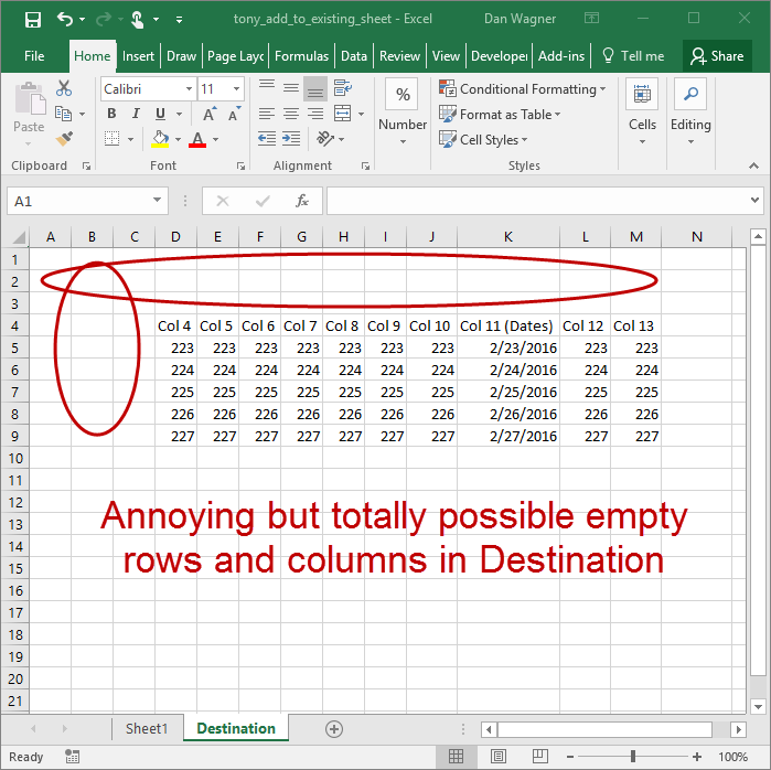
In the remix tradition, though, suppose that the destination block of data is not in the same location as the source data… In fact, what if we don’t even know exactly which column it starts in?
What if our destination is in the middle of nowhere?
Not a problem either. The method we’ll use for identifying the target cell to paste to is totally re-usable in a million other scenarios too!
Just like in the first remix, it’s going to SEEM like a lot of code. It isn’t though — promise.
I can sense you freaking out about how many lines there are here (173) — let’s cut it down to size.
Lines 1-36, just like the remix, are copied from the original tutorial. Code re-use? Love it. That pushes the number of lines down to about 130.
Lines 125-173 were copied from the VBA Toolbelt. You’re using the VBA Toolbelt, right? Re-writing code over and over again is a waste of your precious Analytical know-how — knock that shit off and use the Toolbelt.
That brings us down another 50 lines or so, putting the latest total at ~80.
These last 80 lines are incredibly similar to what we wrote to solve the the challenge in the remix too! The magic in this variation happens on lines 92-106, but let’s not get ahead of ourselves.
The AddToDestinationWorksheet subroutine is where the action’s at. Let’s walk through it using the 4-Step VBA Process as our guide:
Step 1 – Setup is a cinch and takes place from lines 49-51. Here we assign Worksheet variables and also identify the date column.
Step 2 – Exploration is covered by lines 53-59. The goal of this section is to form a Range variable that covers all of the data we’d like to filter — called rngFull in this script. Lines 55 and 56 assign the last-occupied row and column (if you don’t have these functions from the VBA Toolbelt, just do it already. Seriously. I’ll wait…)
Once the last row and last column have been identified, assigning the Range variable is accomplished easily on line 58.
And with that, Exploration is done!
Let’s get into that magic I mentioned above: Step 3 – Execution.
Line 63 sets up a context manager, saving lots of keystrokes while still maintaining readability. (Anything inside the With…End With block that starts with a “.” is applied to rngFull – nice!)
Lines 64-66 wrap up the Range.AutoFilter step. Here’s a quick review of how that works:
Field: the column number, relative to the first column of the Range, that will be filtered (from left to right). Since rngFull starts in column A, the field here is 8 (i.e. column H), but if rngFull started in column C then the field would instead be 5.
Criteria1: the first filter criteria as a String. Since StartDate, our first passed-in variable to AddToDestinationWorksheet, is already a String, a simple concatenation with & works, so if StartDate was set to 3/12/2016 then Criteria1 would be “>=3/12/2016”.
Criteria2: the second filter criteria as a String. Exactly like Criteria1, except this time we are setting this parameter to be less than EndDate (which was the second passed-in variable to AddToDestinationWorksheet). If EndDate was 3/15/2016, then Criteria2 would be “<=3/15/2016”.
Line 70 checks to make sure that the filters were not too severe and that at least one data row remains. It’s a beast, but let’s break this glacier into ice cubes:
wksData.AutoFilter.Range: examine the Range of wksData that has the AutoFilter applied
.Columns(1): of the Range above in #1, examine ONLY the first column
.SpecialCells(xlCellTypeVisible): of the Column above in #2, examine ONLY the cells that are still visible
.Count: return the number of visible cells from the subset defined above in #3
Whew! Since the header row is included in wksData.AutoFilter.Range, the count will always be at least 1. If the count equals 1 after the filter was applied, that means that every data row has been filtered out! This is an uninteresting (and probably unintentional) situation, so we alert the user with a MsgBox on line 72. Lines 74-78 clear any and all filters, and line 79 exits — allowing the user to start again.
Assuming that at least one data row is left, we’re actually going to jump back into Step 2 – Exploration mode from lines 83 to 106! Let’s get after it.
First, we’ll assign all the visible rows, minus the header row, to rngResult on lines 85-87. This variable now owns all the data that must be appended to the Destination Worksheet… which means it’s time to programmatically identify the target Range for our copy / paste!
We start on line 90 by getting the last-occupied row on the Destination Worksheet. Eventually, the paste destination will be one row below the last-occupied row.
Since we don’t know exactly which column to paste to yet, we need to consider two scenarios:
What if the first column is not column A?
What if the first column is column A?
Solving for #1 above takes place on lines 96-100. If the value of the last-occupied row of wksTarget in column A is empty (i.e. vbNullString), we know that column A is NOT the first column. In that case, we solve for lngDestinationFirstCol on lines 97-100:
wksTarget.Range(“A” & lngDestinationLastRow): starts us in the last-occupied row of wksTarget in column A
.End(xlToRight): simulates what happens when you hit CTRL + right arrow on the Excel grid and skips to right until the first occupied cell
.Column: returns the row number of #2 above
Woo! Of course, if the last-occupied row of wksTarget in column A is not empty, that means the data block starts in column A, which means that lngDestinationFirstCol should simply be 1. (This is accomplished on line 102.)
Finally, with lngDestinationFirstCol and lngDestinationLastRow sorted out, we set rngTarget on line 106, remembering to increase lngDestinationLastRow by 1 (since we want to paste immediately below the last-occupied row).
And with that, you have officially handled the second phase Exploration step, which officially wraps up the hard stuff! Take a moment to celebrate how good you look right now.
Looking good you handsome mother flipper!
Last hurrah y’all — back to Execution, and fortunately it’s a one-liner. On line 110, we copy the filtered Range (rngResult) to the destination we just solved for (rngTarget). Smooth!
As always, we wrap up with Step 4 – Cleanup. Lines 115-118 clear filters like a champ, and line 121 lets the user know that our data has been transferred… and with that, you’re done!
Maybe you’re more of a visual learner though — if that’s the case, here’s a 9-minute, multi-example walk through with an emphasis on the magic on lines 92-106:
Is your append-data-to-an-existing-worksheet macro humming along nicely? If not, let me know and I’ll help you get what you need! And if you’d like more step-by-step, no-bullshit VBA guides delivered direct to your inbox, join my email newsletter below.
“152 lines!?” you might have exclaimed to yourself as you came to the end. No argument here — technically, there are 152 lines (including whitespace) in the solution. But let’s cut that WAY down to size.
Lines 1-36, the PromptUserForInputDates subroutine, is exactly what we wrote in the original tutorial. Boom — that brings us down to about 120 lines.
Lines 103-152, the LastOccupiedRowNum and LastOccupiedColNum functions, were pulled directly from the VBA Toolbelt. You’re using the VBA Toolbelt, right? This is exactly the kind of boilerplate the VBA Toolbelt saves you from writing — foundational tasks, like identifying the last-occupied row or last-occupied column on a Worksheet, is something you’ll do thousands of times as an Analyst. Leverage the Toolbelt and save yourself the hassle of rewriting the same code over and over. Boom x2 — that brings us to less than 70 lines. Told ya 🙂
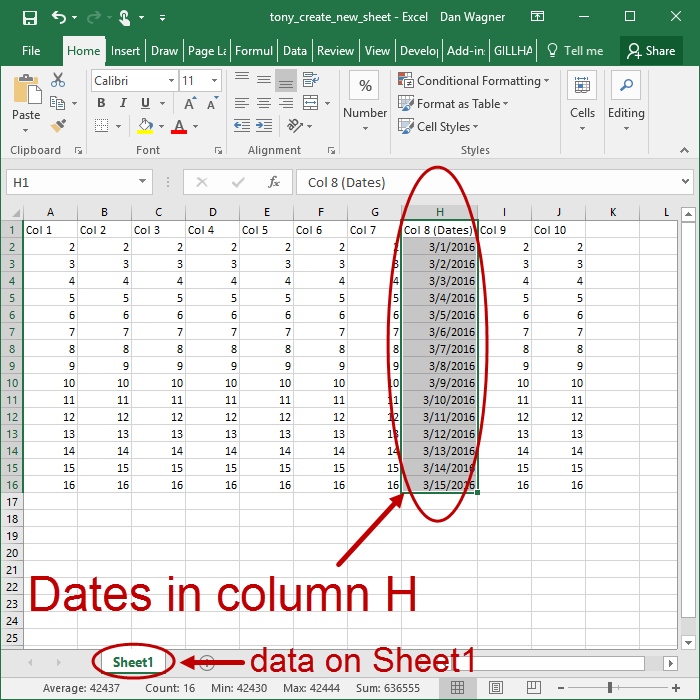
Let’s review CreateSubsetWorksheet, the subroutine that actually copies the data from Sheet1 to a new Worksheet, using the 4-Step VBA Process:
Step 1 – Setup is handled quickly from lines 47 to 48. We assign Sheet1 to a variable and identify the column containing the dates as a number, not a letter (i.e. a string).
Our Step 2 – Exploration takes place on lines 50 to 56. lngLastRow and lngLastCol store the last-occupied row number and last-occupied column number, respectively. Lines 54-56 set up rngFull, which covers all the occupied cells — from the headers in row 1 to the last data row.
Step 3 – Execution is where things get really interesting.
Line 60 starts what is commonly called a “context manager” — With rngFull allows you to save lots of typing without losing ANY clarity, a huge win overall. (After setting the context like this, you can simply type a period character and the VBA editor will open up the expansive list of Range methods, since you are now operating on rngFull.)
Lines 61 to 63 use the amazing Range.AutoFilter method — let’s recap those parameters:
Field: the column number, relative to the first column of the Range, that will be filtered (from left to right). Since rngFull starts in column A, the field here is 8 (i.e. column H), but if rngFull started in column D then the field would instead be 4.
Criteria1: the first filter criteria as a string. Since StartDate is already a String, a simple concatenation with & works, so if StartDate was set to 3/5/2016 then this parameter would be set to “>=3/5/2016”.
Criteria2: the second filter criteria as a String. Exactly like Criteria1, except this time we are setting this parameter to be less than EndDate. If EndDate was 3/10/2016, then this parameter would be set to “<=3/10/2016”.
Range.AutoFilter is a beautiful thing, and after these lines execute the rngFull space has been filtered nicely.
But what if ALL the data was filtered out, say in the case of an incorrect date range entry in the first script? That is an excellent question.
What happens if we filter out everything?
And it’s actually harder than it looks 😐
Since filtering results in a non-continuous block of data, calling Range.Rows will NOT give you what you expect! Write that little factoid down — you WILL forget it at some point (I certainly did), and the note will save you at least an hour of troubleshooting.
So how do you count the number of rows in a filtered Range? It’s a beast, but line 67 shows you the way.
Essentially, this calculation takes the Range that has been filtered (that’s the wksData.AutoFilter.Range part), looks at the first column only (that’s the .Columns(1) part), and counts only the visible cells in that column (that’s the .SpecialCells(xlCellTypeVisible).Count part). This actually makes perfect sense — if you’re only looking at a single column, by counting each visible cell you’re essentially counting each visible row, which is exactly what we want to do here!
If this statement equals 1, we know that rngFull has been completely filtered away and only the header row remains — likely an uninteresting situation to our user. In that case, we throw a message box (on line 69), clear the filters safely (on lines 71-75) and exit the routine (on line 76).
If that beastly statement is greater than 1, though, we know that some rows were left, and that means it’s time to get copying!
Line 82 stores all the visible cells in rngResult. Then, on lines 86 to 87, we create / assign a new Worksheet and create / assign a new Range.
This rngTarget variable will serve as the destination for the copy paste, which takes place on line 88.
Sweet — our data has now been copied to the new Worksheet!
Step 4 – Cleanup, usually short and sweet, is covered by lines 92 to 99.
Clearing filters is absolutely a best practice (leaving them active can lead to pesky run-time errors when rows are unexpectedly hidden), so lines 93 to 96 set the Worksheet.AutoFilterMode parameter to False and call the Worksheet.ShowAllData method (if need be) to obliterate those filters.
Finally, a MsgBox let’s the user know that their data has been transferred on line 99… and that’s it!
If you’re a “seeing is believing” type, here’s a short 6-minute walk through:
Is your script copying a date range to a new Worksheet with ease? If not, let me know and I’ll help you get what you need! And if you’d like more step-by-step, no-bullshit VBA guides delivered direct to your inbox, join my email newsletter below.
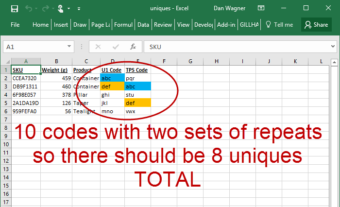
How many times have you heard this old chestnut: “Can you tell me how many unique Xs there are?”
A shitload of times, that’s how many.
Maybe you’ve had success using a formula or a Pivot Table, but the problem gets a whole lot more interesting when you’re stuck with more than one column of data. Let’s fix that with a VBA 1-2 punch:
Use the built-in Collection object to store unique values from anything
Write the results to a new sheet named “uniques-only”
First things first — here’s how to wrap a function around VBA’s Collection and get it to store all uniques.
Interestingly, with this particular function, there is no setup beyond declaring variables. Nice! With that, Step 1 – Setup is complete.
Step 2 – Exploration is very limited in this particular function as well, essentially boils down to a 2-part guard clause from lines 6-11. Let’s talk about both of the cases we’re checking for on line 8.
First, in the case that a Nothing Range is passed in, we want to return a Nothing Collection. What is a Nothing Range, you ask? Good question.
Suppose you declared a Range variable but never assigned it to anything <- THAT is a Nothing Range. Nothing typically occurs when VBA knows about a variable (i.e. Dim rngMyTargetRange As Range), but the variable is never assigned.
We want this function to bulletproof, so lines 8-11 check the passed-in rng to see if it is Nothing. If so, we set the output of the function to col, which has been declared but not assigned to anything (i.e. Nothing) and exit the function.
Second, in the case that a real Range is passed in, but it’s full of blank cells, we also want to return a Nothing Collection. After all, we don’t really care about empty cells — they’re not really unique!
We check the entire rng for “emptiness” by examining the output of WorksheetFunction.CountA(rng), which will be 0 if every cell empty. If that’s the case, we assign the function output to the Nothing col variable and exit, just like we would if rng was Nothing.
Step 3 – Execution is the big one here, and takes place from lines 13 to 35. There’s a lot going on in these ~20 lines, so let’s take it nice and slow.
On line 13, we check to see if the passed-in Range is a single cell. If that’s the case, the returned Collection will be that single value only, so we bind col on line 14 by assigning it to a New Collection and add a single Item to col on line 15. Boom!
When the passed-in Range covers more than one cell (i.e. the vast majority of cases), we get our work done on lines 19-34.
Line 19 assigns the passed-in Range to a Variant array for speedy looping. Line 20 binds col to a New Collection, preparing it to eventually be populated.
On line 24, we tell VBA to ignore errors with On Error Resume Next. Usually, this is to be avoided — but it’s actually critical to this function! We are eventually going to be adding key / value pairs to a Collection in this function. VBA will not add duplicate keys to a Collection, and attempting to do so results in an error — so, by ignoring the error, we’re effectively skipping duplicates!
On line 28, we kick off a loop through everything in the Variant array we created above (on line 19). Since we’re looking for uniques and do not care about the order in which they are collected, the For Each X in Y syntax works beautifully — in each iteration, the variable var contains an element of the Variant array. Smooth!
Finally, our Step 4 – Cleanup takes place on lines 34-38. Line 34 flips errors back on (since we have finished looping through the Variant array), and line 38 ensures that the function returns the uniques-only Collection.
OK awesome — we have a Function that returns a Collection of uniques… it’s time to actually do something with it!
10 codes, 2 repeats, 8 uniques total
If we want to get a single-column list of the uniques across both columns there, the code below will do the trick.
This one is kind of neat in that it goes straight to the user for Step 1 – Setup and Step 2 – Exploration. On line 12 we assign the message we’re going to prompt the user with, and on line 14 we use Application.InputBox (with Type:=8 to allow for a Range selection) to set the target.
You might be asking yourself, “Why is this wrapped in another On Error Resume Next block?”, and like 2Pac I ain’t mad at cha.
“Why do we need an On Error Resume Next block?”
The block allows the user to click “Cancel” error-free and is resolved nicely on line 16, where we check to see if rngTarget is Nothing. (If so, we exit the subroutine.)
The Step 3 – Execution phase is where the magic really happens, and we start on line 19 by using the CollectUniques function we just wrote. This one-liner gives us colUniques, a Collection of all the unique codes that the user selected.
With that, we COULD simply loop through colUniques and write each value out to a new Worksheet. When it comes to writing values to Worksheets, though, I recommend using a Variant array for the performance benefits (since they translate really nicely into Ranges). This example is tiny, but once you have many values the speed will be really noticeable.
On lines 23-26, we fill up a Variant array to make the write process lightning fast. Let’s go line by line here, because there’s a lot going on:
Line 23: we use ReDim to size the Variant array, varUniques, to be a single column that is exactly as long as the Collection of uniques
Line 24: we loop from 1 to the number of uniques in the Collection
Line 25: Variant arrays, interestingly enough, are zero indexed, so we use the index variable (lngIdx) minus one. That zero index applies to the column dimension too, so we’re writing to column number 0!
Phew! In lines 29-31, we add a new Worksheet and take advantage of the fact that Variant arrays can be set to Range for a SUPER fast write. We accomplish this by sizing rngUniques (which will eventually be set to the Variant array from above) along column A, ensuring it is exactly as long as the total number of uniques.
At that point, getting all the values out is as easy as line 31!
Finally, our Step 4 – Cleanup is simply a MsgBox to the user to let him or her know the script has finished. And with that, you’ve got an easy-to-reference, columnar list of uniques!
Want to see the script in action? Check out this 7-minute walk through:
Are you banging out uniques without breaking a sweat? If not, let me know and I’ll help you get what you need! And if you’d like more step-by-step, no-bullshit VBA guides delivered direct to your inbox, join my email newsletter below.