How to Run a Batch File and Wait Until It Finishes with VBA

How do I run a batch file and wait until it finishes with VBA?

Maybe the batch files are from a legacy project, or maybe they’re a short-hand way to accomplish something without needing a scripting language like Python or Ruby — it doesn’t REALLY matter though. Sometimes you just need to run a batch file from VBA!

There are lots of solutions to this problem scattered on Stack Overflow and blogs, but most of them assume that your VBA script does not depend on that results of that batch file operation. What if you need to wait until the batch file finishes though!?

The built-in Windows Script Host Object Model solves this problem for you. First, you’ll need to activate it though.

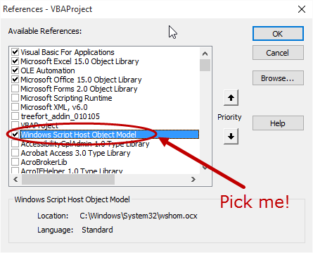
From the VBA window, click Tools > References. In the pop-up window, check the box next to Windows Script Host Object Model:

Make sure the Windows Script Host Object Model is selected

Cool! You know have access to the WshShell object, which will let you WshShell.Run batch files or even regular old CMD commands.

Suppose our batch file is named “Create New 2015 Project Folder.bat” and it’s sitting in C:\wshshell-fun. The following code will run that file and wait for the batch file to finish before moving on.

Here’s a link to the code above so you can review it side-by-side with the walk through below. Right-click, “Open in new window”.

Nice! Here’s a quick run-down of the juicy bits:

Line 10: we use Chr(34) to indicate a double quote character, ". We will need these because the full path to our batch file includes spaces, so variable strCommand becomes:
 
"C:\wshshell-fun\Create New 2015 Project Folder.bat"

Line 11-13: the WshShell.Run command returns a number, so we set it a variable we can later check for errors. (0 is the ideal output from WshShell.Run.)

If you want the operation to happen invisibly, set WindowStyle to 0 — if you actually want to see CMD come up and execute the command, though, you can set WindowStyle:=1 instead.

That final beauty is on Line 13. WaitOnReturn takes True or False — if you want VBA to, you know, WAIT until the command finishes, set it to True!

What if you want to use the some of the old CMD standby commands, like MOVE or REN? In that case, you need to:

1. Prepend your strCommand variable with cmd /K
2. Set WaitOnReturn to False

Let’s say that first, we need to run the batch file. Then, we need to rename the new folder that results from that batch file using some info from cells D3 and E3 on Sheet1. Sound good? Good — here’s the code in action:

Run batch file, wait on results, modify the results

Here’s the code that does it:

Here’s a link to the code above so you can review it side-by-side with the walk through below. Right-click, “Open in new window”.

Sweet! Let’s review how it works with our trusty 4-step VBA process:

Step 1 – Setup
Step 2 – Exploration
Step 3 – Execution
Step 4 – Cleanup

Per usual, we start with Step 1 – Setup. Essentially, this all happens on lines 11-12, where we assign a reference to Sheet1 and store it in the wks variable… easy cheesy.

Step 2 – Exploration is a cinch in this case too and is covered from lines 14-17. From our problem statement, we know that the first part of the intended folder name is in cell D3, and the second part is in cell E3, so we concatenate those values on Line 16 and store the result in strNewFolderName. Progress y’all!

Things get a lot more interesting in our Step 3 – Execution, which takes place from between lines 20-42.

First, from lines 20-29, we apply the same technique we learned above — create a double-quoted string like we’re operating from the command line and run it with WshShell.Run (using the wsh object).

Lines 31-42 get a bit more interesting though, as we need to run the REN CMD command. As mentioned above, when using CMD commands the Run method requires cmd /K to be prepended — which is exactly what we do on line 32. Our trusty Chr(34) is used to wrap the new folder name in double quotes (since it has spaces), and the strNewFolderName variable ALSO has spaces so we wrap it in Chr(34) double quotes too. This time around, we do not wait for a return (since we’re using a built-in CMD command), so line 35 has the WaitOnReturn option set to False.

Finally, Step 4 – Cleanup occurs on line 44, where we prompt the user with a Msgbox to indicate that the job is done. Nice!

Are you running batch files with ease from your VBA code? If not, let me know and I’ll help you get what you need! And if you’d like more step-by-step, no-bullshit VBA guides delivered direct to your inbox, join my email newsletter below.

How to Move Data from Input Sheet to Variable Sheets Based on User Input

How do I move data from one sheet, an input, to a destination sheet picked by the user?

Here’s a challenge that comes up all the time — you built a Workbook with an “input” sheet that lots of people are using. After they enter values on the “input” sheet, they can select where they would like that data to be written by clicking a button, then POOF it moves to the destination they selected.

Here’s what it looks like:

Here’s how our data mover works

But hey, you might be saying… What if the user picks a month for a sheet that does not exist? Like “Aug 2015”? Well, in that case we have some protection built in:

Here’s what our script responds with if the user picks a sheet that does not exist (yet)

Nice! Here’s the code that makes it all work:

Here’s a link to the code above so you can review it side-by-side with the walk through below. Right-click, “Open in new window”.

We will review this macro in the context of our 4-step VBA process, which goes like this:

Step 1 – Setup
Step 2 – Exploration
Step 3 – Execution
Step 4 – Cleanup

As always, we begin with Step 1 – Setup, which is short in this case and only runs from line 12 to line 15. We simply assign the wksAllocate variable to reference the “Allocate” Worksheet, then we collect the user’s drop-down selection and store it in strInput.

The Step 2 – Exploration takes place from line 18 to line 45 and actually accounts for most of this macro. Let’s break it down:

Lines 18-28 make sure that the user’s selection is a Worksheet that exists. We accomplish this by assigning that Worksheet, inside an On Error Resume Next...On Error GoTo 0 block, to an Object. If that assignment results in an error (which is contained in the VBA global variable Err) then we know that Worksheet does not exist — which results in a handy warning message displayed to the user rather than a runtime error.

Once we confirm that the destination Worksheet exists, we assign it to wksTarget on line 31.

Lines 34-39 continue the Step 2 – Exploration by identifying the last-occupied row and column on the “Allocate” Worksheet. Here, we are taking advantage of two functions:

• LastOccupiedRowNum (lines 56-69)
• LastOccupiedColNum (lines 72-86)

These functions do EXACTLY what their names suggest — they return a Long, which represents the last-occupied row or column on the passed-in Worksheet.

(Side note: determining the last-occupied row and last-occupied column on an arbitrary Worksheet is, in my experience, a cornerstone of VBA programming — these handy functions should be a part of any VBA application you are working on.)

Back to lines 34-39. Finally, we assign the Range of data that we would like to cut from the “Allocate” Worksheet to rngAllocate on lines 36-39.

Finally, the last section of Step 2 – Exploration occurs on lines 42-43. Here, we determine the last-occupied row on the target Worksheet, then create a target “destination” Range (rngTaget), which is one row below the last-occupied row on the target Worksheet.

Whew! On to Step 3 – Execution, which is actually a one-liner! Line 46 cuts the data from the “Allocate” Worksheet and pastes it to the destination Worksheet by using the rngTaget we set up on line 43.

Finally, our Step 4 – Cleanup occurs on line 49, where we present the user with a message letting him or her know that the data has been successfully moved.

And with that, our data mover is complete!

Is your data-moving design working smoothly and putting a smile on your users’ faces? If not, let me know and I’ll help you get what you need! And if you’d like more step-by-step, no-bullshit VBA guides delivered direct to your inbox, join my email newsletter below.

How to Copy Data to a New Workbook Based on Dates

How do I copy data between two dates from one workbook to a new workbook?

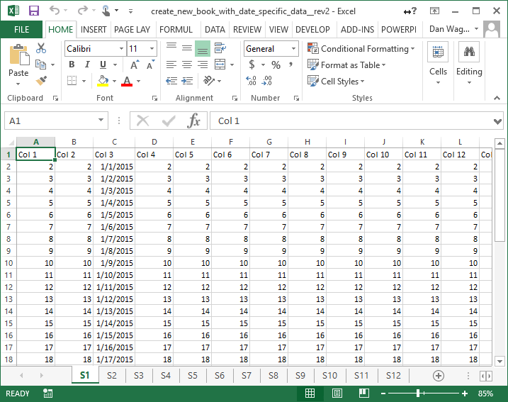
Suppose you have a “master”-type workbook that contains ALL the data for all the dates, spread out amongst many sheets, like this:

Raw Data for ALL dates, spread out onto 12 different sheets

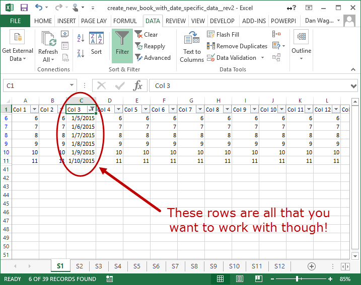
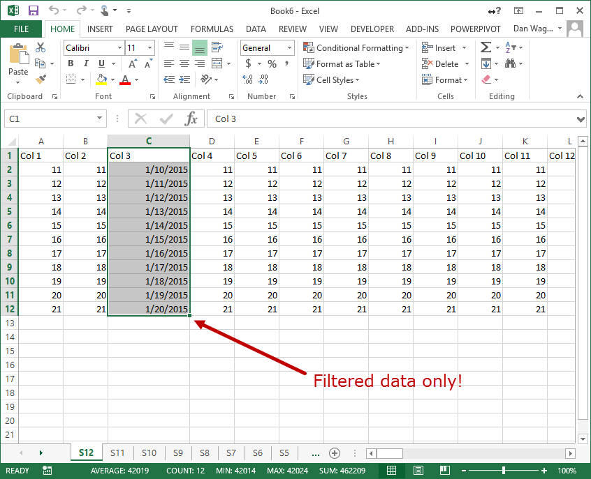
You don’t necessarily need all that data for your analysis — in fact, you are only interested in certain small date range subsets, like, for example, everything that happened between January 5 and January 10:

This is the only block of data you care about on each sheet

How can you get that specific date range of values from each worksheet in a new workbook? You certainly don’t want to filter each sheet by hand… that would take forever! Let’s crack this nut with VBA:

Our macro in action, creating a “subset” workbook with date limits

Woo! Here’s the code that gets it done:

Here’s a link to the code above so you can review it side-by-side with the walk through below. Right-click, “Open in new window”.

Let’s walk through this 2-part code using our 4-step VBA process to guide the way:

Step 1 – Setup
Step 2 – Exploration
Step 3 – Execution
Step 4 – Cleanup

The first subroutine, PromptUserForInptDates, is short but sweet. There is no Step 1 – Setup, Step 2 – Exploration or even Step 4 – Cleanup necessary! It’s all execution here, and beyond that it’s essentially a repeat.

Lines 9-17 prompt the user to input the start date as a String then validate what was entered. For example, if the user puts a non-date into the box, our subroutine will catch the problem and exit instead of creating an error:

This is what happens if your users enters an invalid date

Nice! Unhandled errors are scary to users, and this is a place where we can easily guess what mistakes might happen, so it’s a good idea to go ahead and handle them.

Lines 20-28 do the same thing as lines 9-17 — this time, we get the end date as a String (instead of the start date).

Finally, line 31 calls the CreateSubsetWorkbook subroutine, using the validated-strings we just obtained — now it’s time for the fun stuff!

In a lot of ways, the whole subroutine above PromptUserForInputDates handled MOST of our Step 1 – Setup, but lines 44-45 take care of the final bit. We know the dates are in column C, so we assign lngDateCol to 3. Then, we create a new Workbook and assign it to wbkOutput.

Our Step 2 – Exploration begins inside the loop that we kick off on line 48, which iterates through all the Worksheets inside ThisWorkbook.

First, on lines 52-53, we create a new Worksheet and assign its name to be the same name as the corresponding sheet in ThisWorkbook. Next, on line 57, we create a “target” Range, which is where we’ll paste our filtered data. Then, lines 62-66 find the last-occupied row and column on the sheet, and line 67 assigns the entire data block to our rngFull variable. Woo — now we’re ready for the amazing, built-in Range.AutoFilter method!

Lines 71 through 80 are where the magic happens. We apply the AutoFilter to rngFull, with the following configuration:

1. Field is the column we’re interested in, which we know is 3 (i.e. lngDateCol)
2. Criteria1, which is the first condition we want applied to rngFull, we set to a concatenation of ">= and the StartDate string
3. Criteria2, which is the second condition we want applied to rngFull, we set to a concatenation of "<= and the EndDate string

This gives us a nicely-filtered set of visible cells, which we assign to a “result” variable (rngResult) on line 78. Finally, we copy rngResult to rngTarget, which we set in the beginning of our loop. Boom!

Since we do not want to leave the filters on, lines 83-86 clear all AutoFilter states safely.

Step 4 – Cleanup happens on line 91, which we let the user know that our data has been transferred to the new file.

Our resulting workbook has the right date range ONLY

And with that, we’re done!

Are you masterfully creating new Workbooks with filtered data? If not, let me know and I’ll help you get what you need! And if you’d like more step-by-step, no-bullshit VBA guides delivered direct to your inbox, join my email newsletter below.

How to Transpose Horizontal Data to Vertical Data for Easy Pivot Tables

How do I transpose data from horizontal to vertical to get it ready for a pivot table?

Pivot tables… gotta love ’em. But sometimes your source data just does NOT make sense for a pivot table — and when that’s the case, you need to take matters into your own hands.

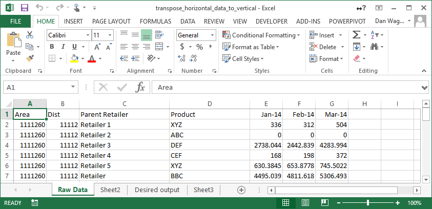
Suppose your raw data looks like this:

Our example data

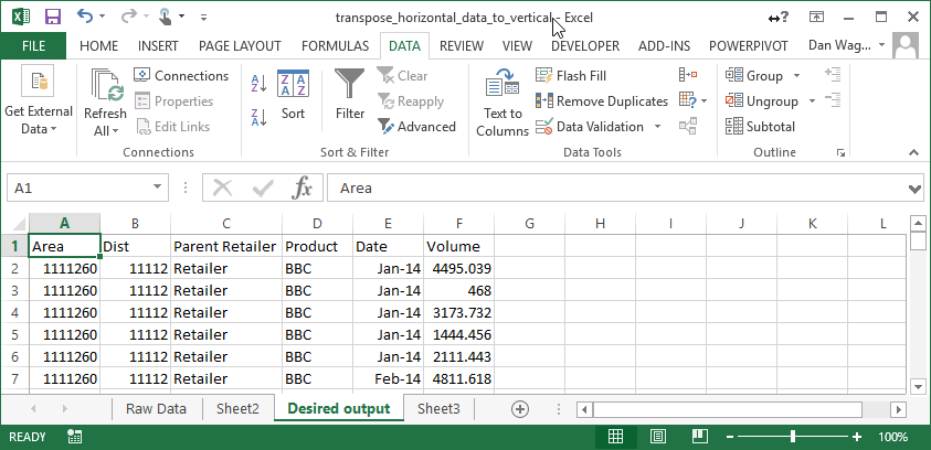
In order to leverage a pivot table here, though, you need to merge the month values (let’s call them “volumes”) into a single column, with the details from the row repeated for each value. In an ideal world, your data would look like this:

This is the way we WANT our data to look

When life gives you lemons, you make lemonade — and VBA is a hell of a lemonade-maker. Before we dive into the code, though, let’s see it in action:

This is our horizontal-to-vertical converting, pivot-preparing macro in action

This script copies the row details, pasting in each month and volume, resulting in an easy-to-pivot block of data. Nice!

One important thing, before we dive into the script itself. This macro relies on Scripting.Dictionary objects, which are not enabled in VBA by default. In order to make them accessible, you need to:

1. Click “Tools” > “References” from the VBA Editor window.
2. Select the “Microsoft Scripting Runtime” option
3. Click “OK”

Enabling the Scripting.Dictionary object for use in VBA

Boom! You now have access to the Scripting.Dictionary, one of the handiest VBA objects around. The Scripting.Dictionary object is a lot like the Collection object, except it has some extra functionality built in. (You can learn a ton about the Scripting.Dictionary object from this Stack Overflow post.

With that out of the way, we can get into the good stuff:

Here’s a link to the code above so you can review it side-by-side with the walk through below. Right-click, “Open in new window”.

Let’s review the above using the always-handy 4-step VBA process:

Step 1 – Setup
Step 2 – Exploration
Step 3 – Execution
Step 4 – Cleanup

Lines 13-23 handle our Step 1 – Setup. First, we assign a Worksheet reference to the “Raw Data” sheet, wksInput. Then we create a new Worksheet reference, where we’ll write the resulting data table, and add headers while we’re at it. Finally, set the starting output row number for the wksOuput sheet in variable lngTargetRow.

Step 2 – Exploration takes place from lines 26-32. In this case, all of the exploration actually occurs on the “Raw Data” sheet, wksInput, so the whole of this step happens inside a With wksInput...End With block:

1. lngLastRow picks up the last-occupied row number
2. varDetailNames is a Variant Array, holding the headers from cell A1 to cell D1
3. varMonthNames is another Variant Array, holding the headers from cell E1 to G1

And that’s it — Exploration complete.

Lines 35-82 handle the Step 3 – Execution, which is the bulk of our macro. There’s a lot in this section, so let’s break it into bite-size pieces…

The outermost loop, which uses lngIdx to iterate through the occupied rows on the “Raw Data” Worksheet, does some setup on lines 37-47. dicDetails and dicValues are initialized and set to new Scripting.Dictionary objects, and two new Variant Arrays are created:

1. varDetails contains the details (like “Area” and “Dist”) for this row
2. varValues contains the values (like 336, 312 and 504) for this row

These two Variant arrays come in handy on lines 51-52, where we call a custom function: CreateDictionaryFromRowArrays. That function is defined and implemented on lines 89-99.

CreateDictionaryFromRowArrays takes Variant Arrays and assembles them into a Scripting.Dictionary, which is exactly what we need in the next step.

Since we want to write the same details (like “Area” and “Dist”) for each value (like 336, 312 or 504), we start by looping through the Keys of the Values dictionary, dicValues, on Line 57. Makes sense, right? We want each value stored in dicValues to be on its own row, so we want that to be our outer loop. (Advanced readers are probably guessing that we’ll be using dicDetails in our inner loop, and that’s EXACTLY our next step.)

Line 63 starts our inner loop, where we write the dicDetails out to each row. Immediately after, on lines 69 and 73, we write the dicValues (which contains one month and one value) out to the same row. Once that is complete, we move on to the next month / value pair inside dicValues, which again is our outer loop.

And that’s it for Step 3 – Execution! By cleverly structuring our Scripting.Dictionary objects, we can write loops that make short work of our horizontal-to-vertical transformation duty.

Finally, line 85 is our one-line Step 4 – Cleanup section, which simply throws the user a message letting him or her know the script is complete. Easy cheesy!

And now, we can whip an unruly data file into a neat, vertical structure that’s primed for analysis with a pivot table. Sweet!

Are you swapping horizontal data for vertical data like a champ? If not, let me know and I’ll help you get what you need! And if you’d like more step-by-step, no-bullshit VBA guides delivered direct to your inbox, join my email newsletter below.