
How to Copy Data Based on Dates: Part 2, an Existing Worksheet

Copying Date Ranges? ALSO TOO GOOD TO BE TRUE
In the first date range-copying remix, we copied a subset of data that matched the user’s dates and pasted it to a new Worksheet in the same Workbook. But what if you need to append that data to an already-existing Worksheet instead?
Easy cheesy y’all — in fact, the code is almost exactly the same.
In the remix tradition, though, suppose that the destination block of data is not in the same location as the source data… In fact, what if we don’t even know exactly which column it starts in?
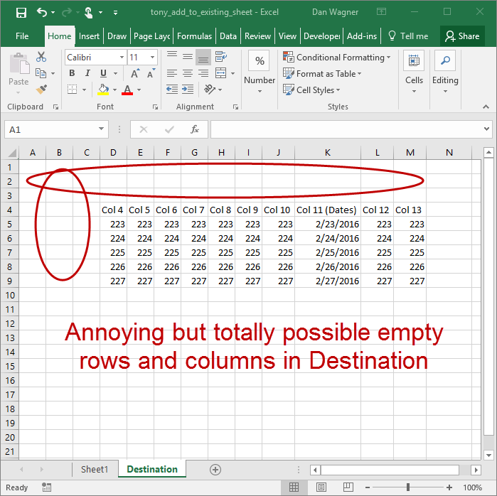
What if our destination is in the middle of nowhere?
Not a problem either. The method we’ll use for identifying the target cell to paste to is totally re-usable in a million other scenarios too!
Just like in the first remix, it’s going to SEEM like a lot of code. It isn’t though — promise.
So take a deep breath and dive in:
I can sense you freaking out about how many lines there are here (173) — let’s cut it down to size.
Lines 1-36, just like the remix, are copied from the original tutorial. Code re-use? Love it. That pushes the number of lines down to about 130.
Lines 125-173 were copied from the VBA Toolbelt. You’re using the VBA Toolbelt, right? Re-writing code over and over again is a waste of your precious Analytical know-how — knock that shit off and use the Toolbelt.
That brings us down another 50 lines or so, putting the latest total at ~80.
These last 80 lines are incredibly similar to what we wrote to solve the the challenge in the remix too! The magic in this variation happens on lines 92-106, but let’s not get ahead of ourselves.
The AddToDestinationWorksheet subroutine is where the action’s at. Let’s walk through it using the 4-Step VBA Process as our guide:
Step 1 – Setup
Step 2 – Exploration
Step 3 – Execution
Step 4 – Cleanup
Step 1 – Setup is a cinch and takes place from lines 49-51. Here we assign Worksheet variables and also identify the date column.
Step 2 – Exploration is covered by lines 53-59. The goal of this section is to form a Range variable that covers all of the data we’d like to filter — called rngFull in this script. Lines 55 and 56 assign the last-occupied row and column (if you don’t have these functions from the VBA Toolbelt, just do it already. Seriously. I’ll wait…)
Once the last row and last column have been identified, assigning the Range variable is accomplished easily on line 58.
And with that, Exploration is done!
Let’s get into that magic I mentioned above: Step 3 – Execution.
Line 63 sets up a context manager, saving lots of keystrokes while still maintaining readability. (Anything inside the With…End With block that starts with a “.” is applied to rngFull – nice!)
Lines 64-66 wrap up the Range.AutoFilter step. Here’s a quick review of how that works:
- Field: the column number, relative to the first column of the Range, that will be filtered (from left to right). Since rngFull starts in column A, the field here is 8 (i.e. column H), but if rngFull started in column C then the field would instead be 5.
- Criteria1: the first filter criteria as a String. Since StartDate, our first passed-in variable to AddToDestinationWorksheet, is already a String, a simple concatenation with & works, so if StartDate was set to 3/12/2016 then Criteria1 would be “>=3/12/2016”.
- Criteria2: the second filter criteria as a String. Exactly like Criteria1, except this time we are setting this parameter to be less than EndDate (which was the second passed-in variable to AddToDestinationWorksheet). If EndDate was 3/15/2016, then Criteria2 would be “<=3/15/2016”.
Line 70 checks to make sure that the filters were not too severe and that at least one data row remains. It’s a beast, but let’s break this glacier into ice cubes:
- wksData.AutoFilter.Range: examine the Range of wksData that has the AutoFilter applied
- .Columns(1): of the Range above in #1, examine ONLY the first column
- .SpecialCells(xlCellTypeVisible): of the Column above in #2, examine ONLY the cells that are still visible
- .Count: return the number of visible cells from the subset defined above in #3
Whew! Since the header row is included in wksData.AutoFilter.Range, the count will always be at least 1. If the count equals 1 after the filter was applied, that means that every data row has been filtered out! This is an uninteresting (and probably unintentional) situation, so we alert the user with a MsgBox on line 72. Lines 74-78 clear any and all filters, and line 79 exits — allowing the user to start again.
Assuming that at least one data row is left, we’re actually going to jump back into Step 2 – Exploration mode from lines 83 to 106! Let’s get after it.
First, we’ll assign all the visible rows, minus the header row, to rngResult on lines 85-87. This variable now owns all the data that must be appended to the Destination Worksheet… which means it’s time to programmatically identify the target Range for our copy / paste!
We start on line 90 by getting the last-occupied row on the Destination Worksheet. Eventually, the paste destination will be one row below the last-occupied row.
Since we don’t know exactly which column to paste to yet, we need to consider two scenarios:
- What if the first column is not column A?
- What if the first column is column A?
Solving for #1 above takes place on lines 96-100. If the value of the last-occupied row of wksTarget in column A is empty (i.e. vbNullString), we know that column A is NOT the first column. In that case, we solve for lngDestinationFirstCol on lines 97-100:
- wksTarget.Range(“A” & lngDestinationLastRow): starts us in the last-occupied row of wksTarget in column A
- .End(xlToRight): simulates what happens when you hit CTRL + right arrow on the Excel grid and skips to right until the first occupied cell
- .Column: returns the row number of #2 above
Woo! Of course, if the last-occupied row of wksTarget in column A is not empty, that means the data block starts in column A, which means that lngDestinationFirstCol should simply be 1. (This is accomplished on line 102.)
Finally, with lngDestinationFirstCol and lngDestinationLastRow sorted out, we set rngTarget on line 106, remembering to increase lngDestinationLastRow by 1 (since we want to paste immediately below the last-occupied row).
And with that, you have officially handled the second phase Exploration step, which officially wraps up the hard stuff! Take a moment to celebrate how good you look right now.

Looking good you handsome mother flipper!
Last hurrah y’all — back to Execution, and fortunately it’s a one-liner. On line 110, we copy the filtered Range (rngResult) to the destination we just solved for (rngTarget). Smooth!
As always, we wrap up with Step 4 – Cleanup. Lines 115-118 clear filters like a champ, and line 121 lets the user know that our data has been transferred… and with that, you’re done!
Maybe you’re more of a visual learner though — if that’s the case, here’s a 9-minute, multi-example walk through with an emphasis on the magic on lines 92-106:
Is your append-data-to-an-existing-worksheet macro humming along nicely? If not, let me know and I’ll help you get what you need! And if you’d like more step-by-step, no-bullshit VBA guides delivered direct to your inbox, join my email newsletter below.